图论算法面试必备：环检测、拓扑排序与DFS/BFS详解

图论是计算机科学中研究图（由节点和边组成）的数学结构的学科，在路径规划、网络分析、任务调度等领域有广泛应用。掌握核心的图论算法，是应对技术面试与解决复杂工程问题的关键。本文将系统性地讲解几种基础的图论算法及其实现，涵盖环检测、拓扑排序、二分图判定，并延伸至并查集、最小生成树和最短路径算法。

图的邻接表表示法

许多图算法都基于邻接表来实现。以下是一个通用的建图函数，适用于表示课程依赖等有向关系。

List<Integer>[] buildGraph(int numCourses, int[][] prerequisites) {
    // 图中共有 numCourses 个节点
    List<Integer>[] graph = new LinkedList[numCourses];
    for (int i = 0; i < numCourses; i++) {
        graph[i] = new LinkedList<>();
    }
    for (int[] edge : prerequisites) {
        int from = edge[1], to = edge[0];
        // 添加一条从 from 指向 to 的有向边
        // 边的方向是「被依赖」关系，即修完课程 from 才能修课程 to
        graph[from].add(to);
    }
    return graph;
}

环检测算法

检测图中是否存在环是许多应用的前提，例如判断任务依赖是否可行。主要有深度优先搜索（DFS）和广度优先搜索（BFS）两种思路。

DFS 实现

DFS通过维护一个递归栈路径（onPath数组）来检测环。如果某个节点在本次递归路径上被重复访问，则说明存在环。

// 记录一次递归堆栈中的节点
boolean[] onPath;
// 记录遍历过的节点，防止走回头路
boolean[] visited;
// 记录图中是否有环
boolean hasCycle = false;

boolean canFinish(int numCourses, int[][] prerequisites) {
    List<Integer>[] graph = buildGraph(numCourses, prerequisites);
    visited = new boolean[numCourses];
    onPath = new boolean[numCourses];
    for (int i = 0; i < numCourses; i++) {
        // 遍历图中的所有节点
        traverse(graph, i);
    }
    // 只要没有循环依赖就可以完成所有课程
    return !hasCycle;
}

void traverse(List<Integer>[] graph, int s) {
    if (onPath[s]) {
        // 出现环
        hasCycle = true;
    }
    if (visited[s] || hasCycle) {
        // 如果已经找到了环，也不用再遍历了
        return;
    }
    // 前序代码位置
    visited[s] = true;
    onPath[s] = true;
    for (int t : graph[s]) {
        traverse(graph, t);
    }
    // 后序代码位置
    onPath[s] = false;
}

BFS 实现（拓扑排序思想）

BFS方法利用拓扑排序的思想，通过计算节点的入度来实现。不断将入度为0的节点从图中移除，如果最终所有节点都能被移除，则说明图中无环。

// 主函数
public boolean canFinish(int numCourses, int[][] prerequisites) {
    // 建图，有向边代表「被依赖」关系
    List<Integer>[] graph = buildGraph(numCourses, prerequisites);
    // 构建入度数组
    int[] indgree = new int[numCourses];
    for (int[] edge : prerequisites) {
        int from = edge[1], to = edge[0];
        // 节点 to 的入度加一
        indgree[to]++;
    }
    // 根据入度初始化队列中的节点
    Queue<Integer> q = new LinkedList<>();
    for (int i = 0; i < numCourses; i++) {
        if (indgree[i] == 0) {
            // 节点 i 没有入度，即没有依赖的节点
            // 可以作为拓扑排序的起点，加入队列
            q.offer(i);
        }
    }
    // 记录遍历的节点个数
    int count = 0;
    // 开始执行 BFS 循环
    while (!q.isEmpty()) {
        // 弹出节点 cur，并将它指向的节点的入度减一
        int cur = q.poll();
        count++;
        for (int next : graph[cur]) {
            indgree[next]--;
            if (indgree[next] == 0) {
                // 如果入度变为 0，说明 next 依赖的节点都已被遍历
                q.offer(next);
            }
        }
    }
    // 如果所有节点都被遍历过，说明不成环
    return count == numCourses;
}

这段 BFS 算法的核心思路如下：

1. 构建邻接表和入度数组。
2. 将入度为 0 的节点入队。
3. 不断弹出队首节点，并将其邻接节点的入度减一，若减为0则入队。
4. 若最终处理的节点数等于总节点数，则无环，反之有环。

拓扑排序算法

对一个有向无环图（DAG）进行拓扑排序，是将所有顶点排成一个线性序列，使得对于任何有向边 (u, v)，u 在序列中都出现在 v 之前。这常用于任务调度、编译顺序确定等场景。

DFS 实现

DFS实现利用后序遍历，拓扑排序结果是后序遍历结果的逆序。

// 记录后序遍历结果
List<Integer> postorder = new ArrayList<>();
// 记录是否存在环
boolean hasCycle = false;
boolean[] visited, onPath;

// 主函数
public int[] findOrder(int numCourses, int[][] prerequisites) {
    List<Integer>[] graph = buildGraph(numCourses, prerequisites);
    visited = new boolean[numCourses];
    onPath = new boolean[numCourses];
    // 遍历图
    for (int i = 0; i < numCourses; i++) {
        traverse(graph, i);
    }
    // 有环图无法进行拓扑排序
    if (hasCycle) {
        return new int[]{};
    }
    // 逆后序遍历结果即为拓扑排序结果
    Collections.reverse(postorder);
    int[] res = new int[numCourses];
    for (int i = 0; i < numCourses; i++) {
        res[i] = postorder.get(i);
    }
    return res;
}

// 图遍历函数
void traverse(List<Integer>[] graph, int s) {
    if (onPath[s]) {
        // 发现环
        hasCycle = true;
    }
    if (visited[s] || hasCycle) {
        return;
    }
    // 前序遍历位置
    onPath[s] = true;
    visited[s] = true;
    for (int t : graph[s]) {
        traverse(graph, t);
    }
    // 后序遍历位置
    postorder.add(s);
    onPath[s] = false;
}

BFS 实现

BFS实现与环检测的BFS算法几乎一致，只是在弹出节点时记录顺序，该顺序即为拓扑排序结果。

// 主函数
public int[] findOrder(int numCourses, int[][] prerequisites) {
    // 建图，和环检测算法相同
    List<Integer>[] graph = buildGraph(numCourses, prerequisites);
    // 计算入度，和环检测算法相同
    int[] indgree = new int[numCourses];
    for (int[] edge : prerequisites) {
        int from = edge[1], to = edge[0];
        indgree[to]++;
    }
    // 根据入度初始化队列中的节点，和环检测算法相同
    Queue<Integer> q = new LinkedList<>();
    for (int i = 0; i < numCourses; i++) {
        if (indgree[i] == 0) {
            q.offer(i);
        }
    }
    // 记录拓扑排序结果
    int[] res = new int[numCourses];
    // 记录遍历节点的顺序（索引）
    int count = 0;
    // 开始执行 BFS 算法
    while (!q.isEmpty()) {
        int cur = q.poll();
        // 弹出节点的顺序即为拓扑排序结果
        res[count] = cur;
        count++;
        for (int next : graph[cur]) {
            indgree[next]--;
            if (indgree[next] == 0) {
                q.offer(next);
            }
        }
    }
    if (count != numCourses) {
        // 存在环，拓扑排序不存在
        return new int[]{};
    }
    return res;
}

二分图判定算法

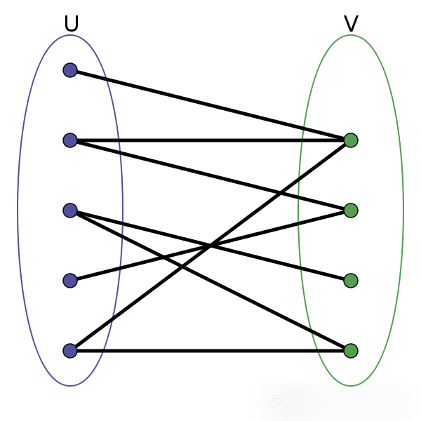
二分图的顶点集可分割为两个互不相交的子集，图中每条边的两个顶点分属于这两个子集，且同一子集内的顶点不相邻。二分图判定问题可以抽象为：能否用两种颜色为图着色，使得任意一条边两端的颜色不同？

DFS 实现

通过DFS遍历，尝试为相邻节点涂上不同颜色，如果冲突则不是二分图。

// 记录图是否符合二分图性质
private boolean ok = true;
// 记录图中节点的颜色，false 和 true 代表两种不同颜色
private boolean[] color;
// 记录图中节点是否被访问过
private boolean[] visited;

// 主函数，输入邻接表，判断是否是二分图
public boolean isBipartite(int[][] graph) {
    int n = graph.length;
    color =  new boolean[n];
    visited =  new boolean[n];
    // 因为图不一定是联通的，可能存在多个子图
    // 所以要把每个节点都作为起点进行一次遍历
    // 如果发现任何一个子图不是二分图，整幅图都不算二分图
    for (int v = 0; v < n; v++) {
        if (!visited[v]) {
            traverse(graph, v);
        }
    }
    return ok;
}

// DFS 遍历框架
private void traverse(int[][] graph, int v) {
    // 如果已经确定不是二分图了，就不用浪费时间再递归遍历了
    if (!ok) return;
    visited[v] = true;
    for (int w : graph[v]) {
        if (!visited[w]) {
            // 相邻节点 w 没有被访问过
            // 那么应该给节点 w 涂上和节点 v 不同的颜色
            color[w] = !color[v];
            // 继续遍历 w
            traverse(graph, w);
        } else {
            // 相邻节点 w 已经被访问过
            // 根据 v 和 w 的颜色判断是否是二分图
            if (color[w] == color[v]) {
                // 若相同，则此图不是二分图
                ok = false;
            }
        }
    }
}

BFS 实现

思路与DFS一致，使用队列进行层次遍历。

// 记录图是否符合二分图性质
private boolean ok = true;
// 记录图中节点的颜色，false 和 true 代表两种不同颜色
private boolean[] color;
// 记录图中节点是否被访问过
private boolean[] visited;

public boolean isBipartite(int[][] graph) {
    int n = graph.length;
    color =  new boolean[n];
    visited =  new boolean[n];

    for (int v = 0; v < n; v++) {
        if (!visited[v]) {
            // 改为使用 BFS 函数
            bfs(graph, v);
        }
    }

    return ok;
}

// 从 start 节点开始进行 BFS 遍历
private void bfs(int[][] graph, int start) {
    Queue<Integer> q = new LinkedList<>();
    visited[start] = true;
    q.offer(start);

    while (!q.isEmpty() && ok) {
        int v = q.poll();
        // 从节点 v 向所有相邻节点扩散
        for (int w : graph[v]) {
            if (!visited[w]) {
                // 相邻节点 w 没有被访问过
                // 那么应该给节点 w 涂上和节点 v 不同的颜色
                color[w] = !color[v];
                // 标记 w 节点，并放入队列
                visited[w] = true;
                q.offer(w);
            } else {
                // 相邻节点 w 已经被访问过
                // 根据 v 和 w 的颜色判断是否是二分图
                if (color[w] == color[v]) {
                    // 若相同，则此图不是二分图
                    ok = false;
                }
            }
        }
    }
}

Union-Find（并查集）算法

当需要频繁判断两个元素是否属于同一集合时，并查集是高效的数据结构。其核心功能是合并（Union）集合与查询（Find）元素所属集合。

核心思想与API

并查集使用树形结构表示集合，根节点作为代表元素。主要API如下：

class UF {
    /* 将 p 和 q 连接 */
    public void union(int p, int q);
    /* 判断 p 和 q 是否连通 */
    public boolean connected(int p, int q);
    /* 返回图中有多少个连通分量 */
    public int count();
}

基础实现

初始化时，每个节点指向自己。合并时，将一个集合的根节点连接到另一个集合的根节点。

class UF {
    // 记录连通分量
    private int count;
    // 节点 x 的父节点是 parent[x]
    private int[] parent;

    /* 构造函数，n 为图的节点总数 */
    public UF(int n) {
        // 一开始互不连通
        this.count = n;
        // 父节点指针初始指向自己
        parent = new int[n];
        for (int i = 0; i < n; i++)
            parent[i] = i;
    }

    public void union(int p, int q) {
        int rootP = find(p);
        int rootQ = find(q);
        if (rootP == rootQ)
            return;
        // 将两棵树合并为一棵
        parent[rootP] = rootQ;
        // parent[rootQ] = rootP 也一样
        count--; // 两个分量合二为一
    }

    /* 返回某个节点 x 的根节点 */
    private int find(int x) {
        // 根节点的 parent[x] == x
        while (parent[x] != x)
            x = parent[x];
        return x;
    }

    public boolean connected(int p, int q) {
        int rootP = find(p);
        int rootQ = find(q);
        return rootP == rootQ;
    }

    public int count() {
        return count;
    }
}

此基础版本find操作最坏时间复杂度为O(N)。

平衡性优化

为避免合并时树退化成链表，引入size数组记录树的节点数（重量），总是将小树接到大树下。

class UF {
    private int count;
    private int[] parent;
    // 新增数组记录树的“重量”
    private int[] size;

    public UF(int n) {
        this.count = n;
        parent = new int[n];
        size = new int[n];
        for (int i = 0; i < n; i++) {
            parent[i] = i;
            size[i] = 1; // 最初每棵树只有一个节点
        }
    }

    public void union(int p, int q) {
        int rootP = find(p);
        int rootQ = find(q);
        if (rootP == rootQ)
            return;
        // 小树接到大树下面，较平衡
        if (size[rootP] > size[rootQ]) {
            parent[rootQ] = rootP;
            size[rootP] += size[rootQ];
        } else {
            parent[rootP] = rootQ;
            size[rootQ] += size[rootP];
        }
        count--;
    }
    // ... find, connected, count 方法
}

优化后时间复杂度降至O(logN)。

路径压缩

进一步优化，使树高保持常数。在find时直接将节点连接到根节点。

// 推荐：递归式路径压缩
public int find(int x) {
    if (parent[x] != x) {
        parent[x] = find(parent[x]);
    }
    return parent[x];
}

使用路径压缩后，union、connected、count操作的平均时间复杂度接近O(1)。通常可省略size优化。

最终推荐实现：

class UF {
    private int count;
    private int[] parent;

    public UF(int n) {
        this.count = n;
        parent = new int[n];
        for (int i = 0; i < n; i++) {
            parent[i] = i;
        }
    }

    public void union(int p, int q) {
        int rootP = find(p);
        int rootQ = find(q);
        if (rootP == rootQ) return;
        parent[rootQ] = rootP;
        count--;
    }

    public boolean connected(int p, int q) {
        return find(p) == find(q);
    }

    public int find(int x) {
        if (parent[x] != x) {
            parent[x] = find(parent[x]);
        }
        return parent[x];
    }

    public int count() {
        return count;
    }
}

应用场景

1. Kruskal最小生成树算法：用于判断加入边是否会形成环。
2. 动态连通性问题：如社交网络好友关系、网络连接状态。
3. 等价类划分：编译器中的变量别名分析等。

Kruskal 最小生成树算法

最小生成树（MST）是连通加权无向图中权重和最小的生成树。Kruskal算法是贪心算法，核心是排序所有边并使用并查集。

算法步骤

1. 将所有边按权重从小到大排序。
2. 依次遍历每条边，若该边连接的两个顶点不在同一连通分量中（用并查集判断），则加入MST并合并这两个分量。
3. 重复步骤2，直到MST包含所有顶点或遍历完所有边。

int minimumCost(int n, int[][] connections) {
    // 城市编号为 1...n，所以初始化大小为 n + 1
    UF uf = new UF(n + 1);
    // 对所有边按照权重从小到大排序
    Arrays.sort(connections, (a, b) -> (a[2] - b[2]));
    // 记录最小生成树的权重之和
    int mst = 0;
    for (int[] edge : connections) {
        int u = edge[0];
        int v = edge[1];
        int weight = edge[2];
        // 若这条边会产生环，则不能加入 mst
        if (uf.connected(u, v)) {
            continue;
        }
        // 若这条边不会产生环，则属于最小生成树
        mst += weight;
        uf.union(u, v);
    }
    // 保证所有节点都被连通
    return uf.count() == 2 ? mst : -1; // 节点0未被使用，占用一个分量
}

复杂度：时间复杂度O(ElogE)（主要来自排序），空间复杂度O(V+E)。

Prim 最小生成树算法

Prim算法也是贪心算法，基于「切分定理」：任意切分中，权重最小的横切边必属于最小生成树。算法从一个顶点开始，逐步扩展MST。

算法实现

使用优先级队列动态维护当前切分的横切边。

class Prim {
    private PriorityQueue<int[]> pq; // 存储横切边
    private boolean[] inMST; // 记录节点是否在MST中
    private int weightSum = 0;
    private List<int[]>[] graph; // 邻接表，边为 {from, to, weight}

    public Prim(List<int[]>[] graph) {
        this.graph = graph;
        int n = graph.length;
        this.pq = new PriorityQueue<>((a, b) -> a[2] - b[2]);
        this.inMST = new boolean[n];
        // 从节点0开始切分
        inMST[0] = true;
        cut(0);
        while (!pq.isEmpty()) {
            int[] edge = pq.poll();
            int to = edge[1];
            int weight = edge[2];
            if (inMST[to]) continue; // 会形成环，跳过
            weightSum += weight;
            inMST[to] = true;
            cut(to); // 新节点加入，进行新一轮切分
        }
    }

    private void cut(int s) {
        for (int[] edge : graph[s]) {
            int to = edge[1];
            if (!inMST[to]) {
                pq.offer(edge);
            }
        }
    }

    public int weightSum() { return weightSum; }
    public boolean allConnected() { /* 检查inMST */ }
}

复杂度：时间复杂度O(ElogE)，空间复杂度O(E)。

Dijkstra 最短路径算法

Dijkstra算法用于计算加权图中单一起点到所有其他节点的最短路径（权重非负）。

算法思想与实现

使用BFS+优先级队列，distTo数组记录最短距离。不同于普通BFS，节点可能被多次访问，但只取距离最小的一次。

class State {
    int id;
    int distFromStart;
    State(int id, int distFromStart) {
        this.id = id;
        this.distFromStart = distFromStart;
    }
}

int[] dijkstra(int start, List<int[]>[] graph) {
    int V = graph.length;
    int[] distTo = new int[V];
    Arrays.fill(distTo, Integer.MAX_VALUE);
    distTo[start] = 0;
    PriorityQueue<State> pq = new PriorityQueue<>((a, b) -> a.distFromStart - b.distFromStart);
    pq.offer(new State(start, 0));

    while (!pq.isEmpty()) {
        State curState = pq.poll();
        int curNodeID = curState.id;
        int curDistFromStart = curState.distFromStart;
        if (curDistFromStart > distTo[curNodeID]) {
            continue; // 已有更优路径
        }
        for (int[] edge : graph[curNodeID]) {
            int nextNodeID = edge[1];
            int weight = edge[2];
            int distToNextNode = distTo[curNodeID] + weight;
            if (distTo[nextNodeID] > distToNextNode) {
                distTo[nextNodeID] = distToNextNode;
                pq.offer(new State(nextNodeID, distToNextNode));
            }
        }
    }
    return distTo;
}

若只求起点到终点的距离，可在从队列中取出节点时判断是否为终点。

A* 搜索算法

A*是启发式搜索算法，结合了Dijkstra的完备性和贪心搜索的效率，用于已知目标节点的路径规划。在技术面试尤其是LeetCode等算法平台中，理解其与BFS、Dijkstra的区别至关重要。

核心思想

A*定义评估函数 f(n) = g(n) + h(n)：

• g(n)：从起点到节点n的实际代价。
• h(n)：从节点n到目标点的预估代价（启发函数）。
  算法优先探索f(n)值最小的节点。

启发函数选择

常见的启发函数（用于网格地图）有：

1. 曼哈顿距离：d = |x1-x2| + |y1-y2|
2. 欧几里得距离：d = sqrt((x1-x2)^2 + (y1-y2)^2)
3. 切比雪夫距离：d = max(|x1-x2|, |y1-y2|)

代码实现（欧几里得距离）

class Node {
    int x, y;
    double gCost, hCost, fCost;
    Node parent;
    public Node(int x, int y) { this.x = x; this.y = y; }
    public double calculateHeuristic(Node target) {
        return Math.sqrt(Math.pow(x - target.x, 2) + Math.pow(y - target.y, 2));
    }
    public void updateCosts(Node target, double gCost) {
        this.gCost = gCost;
        this.hCost = calculateHeuristic(target);
        this.fCost = this.gCost + this.hCost;
    }
    // 重写 equals 和 hashCode
}

class AStar {
    private static final int[][] DIRECTIONS = {{1,0},{-1,0},{0,1},{0,-1},{1,1},{1,-1},{-1,1},{-1,-1}};
    public List<Node> findPath(Node start, Node target, int[][] grid) {
        Set<Node> openSet = new HashSet<>();
        Set<Node> closedSet = new HashSet<>();
        PriorityQueue<Node> pq = new PriorityQueue<>(Comparator.comparingDouble(n -> n.fCost));
        start.updateCosts(target, 0);
        openSet.add(start);
        pq.add(start);
        while (!openSet.isEmpty()) {
            Node current = pq.poll();
            openSet.remove(current);
            closedSet.add(current);
            if (current.equals(target)) {
                return reconstructPath(current);
            }
            for (int[] dir : DIRECTIONS) {
                int newX = current.x + dir[0], newY = current.y + dir[1];
                if (!isInBounds(newX, newY, grid) || grid[newX][newY] == 1) continue;
                Node neighbor = new Node(newX, newY);
                if (closedSet.contains(neighbor)) continue;
                double tentativeGCost = current.gCost + current.calculateHeuristic(neighbor);
                if (!openSet.contains(neighbor) || tentativeGCost < neighbor.gCost) {
                    neighbor.updateCosts(target, tentativeGCost);
                    neighbor.parent = current;
                    if (!openSet.contains(neighbor)) {
                        openSet.add(neighbor);
                        pq.add(neighbor);
                    }
                }
            }
        }
        return Collections.emptyList();
    }
    private boolean isInBounds(int x, int y, int[][] grid) { ... }
    private List<Node> reconstructPath(Node node) { ... }
}

对比与总结

• BFS：无权图最短路径，时间复杂度O(V+E)。
• Dijkstra：带权非负图最短路径，保证最优，但可能探索过多节点。
• **A*：有明确目标点的路径搜索，通过启发函数引导方向，效率通常更高，在启发函数可采纳（估计值不大于真实值）时保证最优解**。
• 局限性：A需要明确的目标点。对于多目标找最近或未知目标搜索，Dijkstra或BFS更合适。A的空间消耗可能较高，对此有IDA*等优化变种。

掌握这些基础图论算法及其实现，能够帮助开发者有效解决涉及图结构数据的复杂问题，是提升算法与数据结构能力的核心环节。从环检测、拓扑排序到最短路径规划，理解其背后的DFS、BFS以及并查集思想，并能在不同场景下选择合适的算法，是进行高效、可靠系统设计与开发的重要基础。