在预测学生考试通过率的场景中,我们常常拥有复习时长、作业完成率等多个特征。一种强大的建模思想是集成学习,即组合多个“弱”模型来共同决策,从而形成一个强模型。
XGBoost 是梯度提升树(Gradient Boosting Decision Tree, GBDT)的一种高效实现,其核心思想可以概括为:
- 从一个简单的初始猜测开始(例如,认为所有学生通过的概率都是0.6)。
- 找出预测错误的样本,将这些误差(残差)作为新的目标,训练一棵小决策树来修正这些错误。
- 将这棵小树的预测值加到初始预测上,得到更新后的预测结果。
- 重复上述过程:每一轮都训练一棵新树,专门学习之前所有树累积预测的残差。
- 最终将所有树的预测贡献相加(通常乘以一个学习率以控制步长),得到最终的预测值。
XGBoost 在传统梯度提升树的基础上进行了关键改进:它利用二阶导(Hessian)信息来更精确地计算每次迭代的修正量,并引入正则化项来防止过拟合。在寻找决策树的最佳分裂点时,它采用了高效的增益计算公式。这些特性使得 XGBoost 通常比基础版本更快、更稳定,且泛化能力更强。
下面我们用公式来精确描述在二分类任务中,每一轮用于拟合的目标。假设模型当前对样本 i 的预测值为 $F_i$(即对数几率,log-odds),则预测概率为 $p_i = \\sigma(F_i)$,其中 $\\sigma$ 是 sigmoid 函数。给定真实标签 $y_i \\in \\{0,1\\}$,我们可以计算损失函数的一阶导(梯度,g)和二阶导(海森矩阵,h):
$g_i = \\frac{\\partial l(y_i, p_i)}{\\partial F_i} = p_i - y_i$
$h_i = \\frac{\\partial^2 l(y_i, p_i)}{\\partial F_i^2} = p_i(1-p_i)$
对于决策树某个叶子节点上的所有样本,我们将其一阶梯度和 $G$ 与二阶梯度和 $H$ 分别求和。XGBoost 会为该叶子节点计算一个最优的输出权重 $w$:
$w^* = -\\frac{G}{H + \\lambda}$
其中 $\\lambda$ 是控制叶子权重的 L2 正则化系数。
在决定是否分裂一个节点时,XGBoost 使用以下增益公式来衡量分裂的收益:
$Gain = \\frac{1}{2} \\left[ \\frac{G_L^2}{H_L + \\lambda} + \\frac{G_R^2}{H_R + \\lambda} - \\frac{(G_L+G_R)^2}{H_L+H_R + \\lambda} \\right] - \\gamma$
其中,$G_L, H_L$ 和 $G_R, H_R$ 分别是分裂后左、右子节点的一阶和二阶梯度和,$\\gamma$ 是控制分裂复杂度的惩罚项。选择能使增益最大化的特征和阈值进行分裂。
这就是 XGBoost 的核心精髓:利用一阶梯度(Gradient)和二阶海森矩阵(Hessian)信息来共同决定决策树叶子的权重以及分裂点,从而实现更快的收敛速度和更高的模型稳定性。 这种基于二阶泰勒展开的优化思想,使其在众多集成学习算法中脱颖而出。
完整案例与代码实现
下面我们通过一个完整的示例来演示 XGBoost 风格模型的构建过程。案例将包含以下步骤:
- 构造一个非线性可分的合成二分类数据集。
- 使用 PyTorch 实现基于 XGBoost 增益公式的树结构(包含一阶、二阶信息处理)。
- 训练模型并记录损失、准确率及特征重要性。
import numpy as np
import torch
import matplotlib.pyplot as plt
from matplotlib import cm
torch.set_default_dtype(torch.float32)

# 生成合成数据(两个簇 + 非线性分布)
def make_synthetic(n=500, noise=0.2, seed=42):
    np.random.seed(seed)
    t = np.random.rand(n) * 2 * np.pi
    r = 1.0 + noise * np.random.randn(n)
    x1 = r * np.cos(t)
    y1 = r * np.sin(t)
# 一个环状簇 + 中间簇
    x2 = 0.4 * np.random.randn(n)
    y2 = 0.4 * np.random.randn(n)
    X = np.vstack([np.column_stack([x1, y1]),
                   np.column_stack([x2+1.5, y2])])
    y = np.hstack([np.ones(n), np.zeros(n)])
# 打乱
    idx = np.random.permutation(len(y))
    X = X[idx]; y = y[idx]
    return torch.tensor(X, dtype=torch.float32), torch.tensor(y, dtype=torch.float32)

X, y = make_synthetic(n=1000, noise=0.15)
N, D = X.shape

# Sigmoid helper
def sigmoid(x): return 1.0 / (1.0 + torch.exp(-x))

# 决策树结点(用于回归的基学习器,基于 XGBoost 的增益计算)
class XGNode:
    def __init__(self, depth=0):
        self.depth = depth
        self.is_leaf = False
        self.feature = None
        self.threshold = None
        self.left = None
        self.right = None
        self.weight = 0.0 # 叶子权重
        self.gain = 0.0

class XGTree:
    def __init__(self, max_depth=3, min_samples_split=10, lamb=1.0, gamma=0.0):
        self.max_depth = max_depth
        self.min_samples_split = min_samples_split
        self.lamb = lamb
        self.gamma = gamma
        self.root = None
        self.feature_gains = None

    def fit(self, X, g, h):
# X: torch [N, D], g,h: torch [N]
        self.feature_gains = np.zeros(X.shape[1], dtype=float)
        idx_all = torch.arange(X.shape[0])
        self.root = self._build_node(X, g, h, idx_all, depth=0)

    def _build_node(self, X, g, h, idx, depth):
        node = XGNode(depth=depth)
        G = g[idx].sum().item(); H = h[idx].sum().item()
# 叶子权重(XGBoost 解析解)
        node.weight = -G / (H + self.lamb)
# 若满足停止条件,则成为叶子
        if depth >= self.max_depth or idx.shape[0] <= self.min_samples_split:
            node.is_leaf = True
            return node
        best_gain = 0.0
        best_feature, best_thr = None, None
        best_left_idx, best_right_idx = None, None
# 尝试每个特征的分裂
        for j in range(X.shape[1]):
            xj = X[idx, j]
# 提取候选阈值(使用排序中间点)
            vals, perm = torch.sort(xj)
            g_sorted = g[idx][perm]
            h_sorted = h[idx][perm]
# 计算 prefix sums
            G_left = torch.cumsum(g_sorted, dim=0)[:-1].numpy()
            H_left = torch.cumsum(h_sorted, dim=0)[:-1].numpy()
            G_total = G
            H_total = H
# thresholds 是中点 between consecutive unique values
            vals_np = vals.numpy()
            thr_candidates = (vals_np[:-1] + vals_np[1:]) / 2.0
# 遍历阈值位置
            if len(thr_candidates) == 0:
                continue
# compute gains vectorized
            G_right = G_total - G_left
            H_right = H_total - H_left
# Avoid tiny splits
            valid = (np.arange(len(thr_candidates)) > 0) & (G_right.size>0)
# compute gain for each split
            gain = 0.5 * ( (G_left**2)/(H_left + self.lamb) + (G_right**2)/(H_right + self.lamb) - (G_total**2)/(H_total + self.lamb) ) - self.gamma
# Pick max
            idx_max = np.nanargmax(gain)
            if gain[idx_max] > best_gain:
                best_gain = float(gain[idx_max])
                best_feature = j
                best_thr = float(thr_candidates[idx_max])
# Build left/right indices based on threshold
                left_mask = (X[:, j] <= best_thr)
# restrict to current idx set
                idx_local = idx[left_mask[idx]]
                right_mask = (X[:, j] > best_thr)
                idx_right_local = idx[right_mask[idx]]
                best_left_idx = idx_local
                best_right_idx = idx_right_local
        if best_feature is None or best_gain <= 0:
            node.is_leaf = True
            return node
# 记录特征重要度(用增益累计)
        self.feature_gains[best_feature] += best_gain
        node.feature = best_feature
        node.threshold = best_thr
        node.gain = best_gain
        node.left = self._build_node(X, g, h, best_left_idx, depth+1)
        node.right = self._build_node(X, g, h, best_right_idx, depth+1)
        return node

    def _predict_one(self, x, node):
        if node.is_leaf:
            return node.weight
        if x[node.feature] <= node.threshold:
            return self._predict_one(x, node.left)
        else:
            return self._predict_one(x, node.right)

    def predict(self, X):
        out = []
        for i in range(X.shape[0]):
            out.append(self._predict_one(X[i], self.root))
        return torch.tensor(out, dtype=torch.float32)

# XGBoost 风格的提升器
class SimpleXGBoost:
    def __init__(self, n_estimators=30, lr=0.3, max_depth=3, lamb=1.0, gamma=0.0):
        self.n_estimators = n_estimators
        self.lr = lr
        self.trees = []
        self.max_depth = max_depth
        self.lamb = lamb
        self.gamma = gamma
        self.init_score = 0.0
        self.feature_importances_ = None

    def fit(self, X, y):
        N = X.shape[0]
# 初始化 F0 为 log(odds)
        p0 = y.mean().item()
        self.init_score = np.log((p0+1e-12)/(1-p0+1e-12))
        F = torch.full((N,), fill_value=self.init_score)
        self.trees = []
        losses = []
        accs = []
        for m in range(self.n_estimators):
            p = sigmoid(F)
            g = p - y
            h = p * (1 - p)
            tree = XGTree(max_depth=self.max_depth, lamb=self.lamb, gamma=self.gamma)
            tree.fit(X, g, h)
            pred = tree.predict(X)
            F = F + self.lr * pred
            self.trees.append(tree)
# 评价指标
            p_new = sigmoid(F)
# log loss
            eps = 1e-12
            loss = -(y*torch.log(p_new+eps) + (1-y)*torch.log(1-p_new+eps)).mean().item()
            pred_label = (p_new>0.5).float()
            acc = (pred_label == y).float().mean().item()
            losses.append(loss); accs.append(acc)
# early stop(可选)
# print(m, loss, acc)
# 合并特征重要度
        fi = np.zeros(X.shape[1])
        for t in self.trees:
            if t.feature_gains is not None:
                fi += t.feature_gains
        self.feature_importances_ = fi / (fi.sum() + 1e-12)
        return losses, accs

    def predict_proba(self, X):
        F = torch.full((X.shape[0],), fill_value=self.init_score)
        for t in self.trees:
            F = F + self.lr * t.predict(X)
        p = sigmoid(F).numpy()
        return np.vstack([1-p, p]).T

    def predict(self, X):
        probs = self.predict_proba(X)[:,1]
        return (probs>0.5).astype(int)
代码解析:
- 数据生成:我们生成了两个簇,一个呈环状分布,一个集中在中心,构成一个非线性可分的任务,便于考察决策树模型的非线性拟合能力。
- XGNode / XGTree:我们实现了一棵用于回归的树,但其分裂依据不是传统的均方误差(MSE),而是 XGBoost 的增益公式。对于每个候选分裂点,计算左右子集的一阶和二阶导数和,代入增益公式评估分裂收益。叶节点的权重采用解析解
$w^* = -G/(H+\\lambda)$,这是 XGBoost 的关键,它让每个叶子的输出值考虑了二阶信息,而不仅仅是残差的平均值。
- SimpleXGBoost:管理整个提升过程。初始化预测值为所有样本的对数几率
$F_0$。在每一轮迭代中,计算当前预测概率 $p$、梯度 $g$ 和 Hessian $h$,然后将 $(g, h)$ 传给 XGTree 去构建一棵新树来拟合这些目标。训练过程中会记录每轮的损失和准确率。
模型可视化与分析
训练完成后,我们可以通过一系列图表来直观评估模型表现。
# 训练并记录
model = SimpleXGBoost(n_estimators=30, lr=0.5, max_depth=3, lamb=1.0, gamma=0.0)
losses, accs = model.fit(X, y)

# 1) 数据分布与决策边界
xx = np.linspace(X[:,0].min()-0.5, X[:,0].max()+0.5, 300)
yy = np.linspace(X[:,1].min()-0.5, X[:,1].max()+0.5, 300)
grid = torch.tensor(np.array(np.meshgrid(xx, yy)).T.reshape(-1,2), dtype=torch.float32)
proba = model.predict_proba(grid)[:,1].reshape(300,300)

plt.figure(figsize=(8,6))
plt.contourf(xx, yy, proba, levels=20, cmap=cm.viridis, alpha=0.7)
# 数据点
pos = (y.numpy()==1)
plt.scatter(X[pos,0].numpy(), X[pos,1].numpy(), c='orange', edgecolor='k', label='class 1', s=30)
plt.scatter(X[~pos,0].numpy(), X[~pos,1].numpy(), c='deepskyblue', edgecolor='k', label='class 0', s=30)
plt.title("决策边界与数据点(颜色越暖,预测为 class 1 概率越高)")
plt.legend()
plt.colorbar(label='P(class=1)')
plt.show()

# 2) 训练曲线(loss & accuracy)
plt.figure(figsize=(8,4))
plt.plot(losses, label='logloss', color='magenta', linewidth=2)
plt.xlabel('迭代次数(树的数量)'); plt.ylabel('log-loss')
plt.twinx()
plt.plot(accs, label='accuracy', color='limegreen', linewidth=2)
plt.ylabel('accuracy')
plt.title('训练曲线:loss & accuracy')
plt.show()

# 3) 特征重要性
fi = model.feature_importances_
plt.figure(figsize=(6,4))
plt.bar(range(len(fi)), fi, color=['#FF6F61', '#6B5B95'])
plt.xticks([0,1], ['feature 0', 'feature 1'])
plt.title('特征重要性(基于增益累计)')
plt.show()

# 4) 预测概率按真实类的分布(直方图)
probs_train = model.predict_proba(X)[:,1]
plt.figure(figsize=(8,4))
plt.hist(probs_train[y.numpy()==1], bins=30, alpha=0.7, label='true=1', color='tomato')
plt.hist(probs_train[y.numpy()==0], bins=30, alpha=0.7, label='true=0', color='royalblue')
plt.title('预测概率分布:不同真类样本的概率密度')
plt.xlabel('P(class=1)')
plt.legend()
plt.show()
决策边界图:
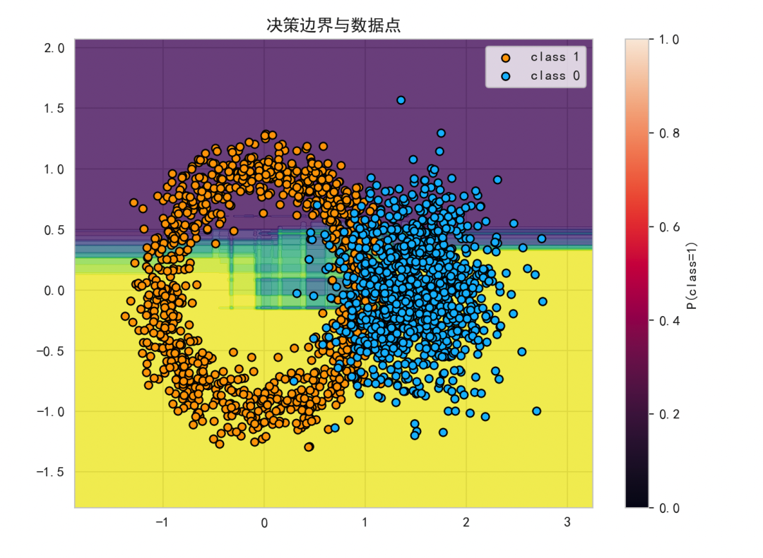
图中暖色区域表示模型预测为 class 1 的概率较高。该图直观展示了多棵决策树组合如何划分出复杂的非线性边界(如环状)。如果模型容量足够且未过拟合,边界会贴合数据的真实分布。
训练曲线:
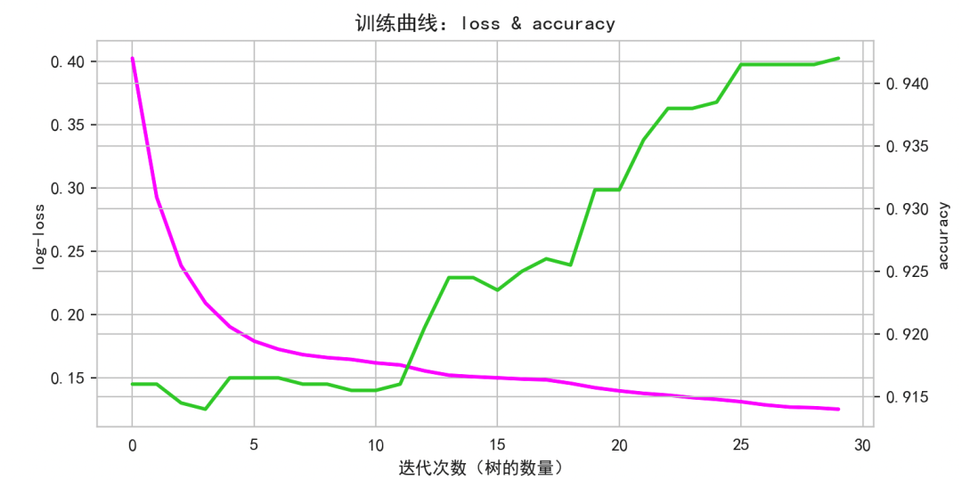
左轴为对数损失(log-loss),右轴为准确率(accuracy)。通常随着树的数量增加,损失快速下降后趋于平缓,准确率则上升后稳定。通过此曲线可以判断模型是否收敛,以及是否需要调整学习率或增加树的数量。
特征重要性:
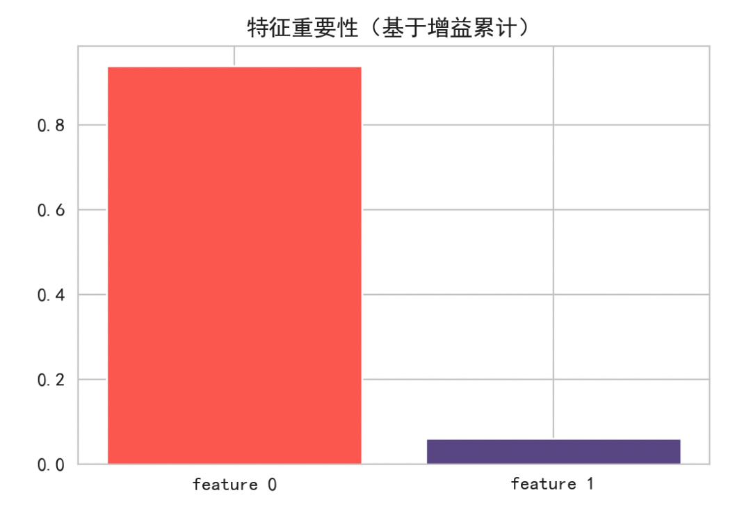
柱状图展示了每个特征在所有树的分裂中带来的总增益。如果某个特征的重要性显著高于其他特征,说明模型更多地依赖该特征进行决策,这为特征筛选提供了依据。
预测概率分布:
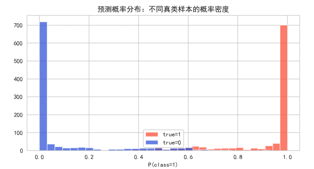
理想情况下,正类样本(true=1)的预测概率应集中在1附近,负类样本(true=0)的概率应集中在0附近。若两者分布重叠严重,则表明模型的区分能力有限,可能需要调整模型或进行概率校准。
关键调参要点
在实际使用 XGBoost 时,以下几个超参数对模型性能影响显著:
- 学习率 (lr):控制每棵树对最终预测的贡献程度。较小的学习率使模型更稳健,但需要训练更多的树(增加时间和复杂度)。常见范围在 0.01 到 0.3 之间。
- 树的数量 (n_estimators):与学习率紧密相关。学习率较小时,需要更多的树来达到相同的拟合效果。两者需配合调整。
- 树的最大深度 (max_depth):控制单棵树的复杂度。深度越大,模型学习非线性关系的能力越强,但也越容易过拟合。常用值在 3 到 10 之间。
- 正则化参数 (lamb 和 gamma):
lambda (或 reg_lambda) 是 L2 正则化项,控制叶子权重的平滑度;gamma (或 min_split_loss) 是分裂所需的最小损失下降,用于控制树的生长。合理设置能有效抑制过拟合。
- 早停法 (early stopping):在独立的验证集上监控评估指标(如 log-loss),当指标在连续多轮迭代中不再提升时,提前终止训练。这是防止过拟合的实用技巧。
总结
XGBoost 的强大性能主要源于其对二阶信息(Hessian)的利用和有效的模型复杂度控制(正则化)。前者使其能够更精确、更快速地逼近目标函数,后者则保障了模型具有良好的泛化能力,避免过拟合。
本文通过原理阐述、公式推导,并结合一个使用 PyTorch 从零实现的示例,完整地展示了 XGBoost 的核心思想。我们不仅实现了基于二阶导数的树结构生长和叶子权重计算,还通过决策边界、训练曲线、特征重要性等多角度对模型进行了可视化分析,希望能帮助大家更深入地理解这一经典且强大的梯度提升树算法。
如果你想探讨更多关于机器学习实践或算法实现的细节,欢迎访问云栈社区与其他开发者交流。
 发表于 2026-3-10 14:57:34
|
查看: 121|
回复: 0
发表于 2026-3-10 14:57:34
|
查看: 121|
回复: 0
