
很多人接触概率交易,往往从一个非常简单的直觉开始:一个事件有多大概率发生。
但在真正的量化交易台上,这个问题会逐渐演化成一整套复杂的模拟体系。从最简单的抛硬币模型,到 Monte Carlo模拟、尾部风险估计、实时粒子滤波,再到多层次的方差控制技术,咱们将一步步探索这个问题的核心——“如何像量化交易员一样进行模拟?”
如果按顺序阅读,你会看到每一层模型是如何自然衔接起来的,并最终构成量化交易桌日常使用的模拟工具链。
本文仅用于研究与技术学习,不构成任何投资建议,请独立研究并自行判断。

1. 决定一切的“抛硬币模型”
假设你正在查看 Polymarket 上的一个合约:
“美联储是否会在3月降息?”
YES 合约价格为 $0.62。
很多交易者会很自然地这样理解:
市场认为降息概率是 62%。
如果你的判断是 70%,那么结论似乎很简单: 买入。
事实上,这正是绝大多数散户交易者的思考方式。
他们把预测市场合约理解为一枚带偏置的硬币: 市场给出概率 -> 自己重新估计概率 -> 交易两者之间的差值
问题在于,这个思路忽略了大量关键因素。例如:
- 你的 70% 置信度有多高
- 明天的 就业数据公布 会如何改变概率
- Polymarket 上其他 与美联储相关的合约之间的相关性
- 在最终结果揭晓之前,价格路径是否允许你获利退出
如果只是抛硬币,模型只有一个参数。但一个现实的预测市场合约背后却包含大量维度,预测市场合约嵌入到一系列相关事件的组合中,具有随时间变化的信息流、订单簿动态和执行风险,有几十种。
也正是因为这些复杂性,量化交易台需要依赖更系统的 概率模拟框架。
2. 蒙特卡洛,许多人忽视的基础
几乎所有复杂的模拟系统,最终都会回到一个核心方法:
Monte Carlo Simulation
基本思想非常简单:
- 从概率分布中抽样
- 计算结果
- 重复很多次
- 用样本平均估计概率
如果事件为 $X$,概率为 $p$。
Monte Carlo估计量为 $\hat{p} = \frac{1}{N} \sum_{i=1}^{N} \mathbf{1}(X^{(i)} = 1)$。
根据中心极限定理,估计误差收敛速度为 $O(N^{-1/2})$。
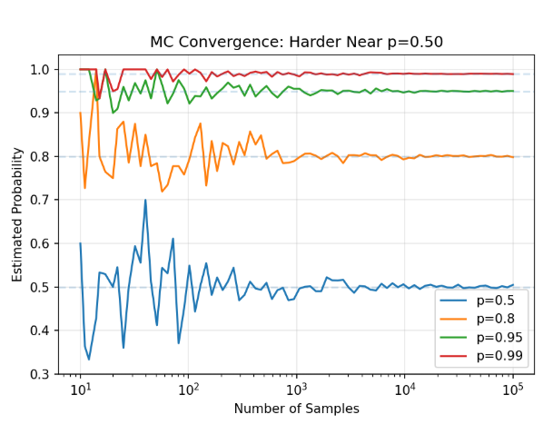
其方差为 $\text{Var}(\hat{p}) = p(1-p)/N$。
因此,
当 p = 0.5 时,方差最大。
换句话说,价格在50美分附近的预测合约反而最难估计。
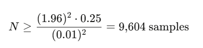
如果希望在 95%置信水平下达到 ±0.01 精度,当 $p = 0.5$ 时需要大约:
10,000 次模拟。
对于简单问题,这个规模完全可以接受。
但当我们开始模拟 价格路径 而不是终点时,复杂度会迅速增加。
实验模拟
假设我们需要评估一个资产相关的二元合约,例如:
“AAPL 是否会在3月15日前收盘高于 $200?”
可以使用 Geometric Brownian Motion 模拟终端价格。
目标: 估计与资产挂钩的二元合约实现盈利的概率(例如,“苹果公司股价在 3 月 15 日之前能否收于 200 美元以上?”)
示例代码如下:
import numpy as np

def simulate_binary_contract(S0, K, mu, sigma, T, N_paths=100_000):

    Z = np.random.standard_normal(N_paths)

    S_T = S0 * np.exp(
        (mu - 0.5 * sigma**2) * T +
        sigma * np.sqrt(T) * Z
    )

    payoffs = (S_T > K).astype(float)

    p_hat = payoffs.mean()

    se = np.sqrt(p_hat * (1 - p_hat) / N_paths)
对于 单一资产、单一合约、对数正态假设,这个模型已经可以工作。
但现实世界的预测市场几乎会破坏所有这些假设。
如何评估模拟质量
在改进模拟之前,需要先解决一个问题:
如何评估概率预测是否可靠?
预测市场和概率模型通常使用 Brier Score 来评估校准程度:
$BS = \frac{1}{N} \sum_{i=1}^N (f_i - o_i)^2$,其中 $f_i$ 是预测概率,$o_i$ 是实际结果 (0/1)。
示例代码:
def brier_score(predictions, outcomes):
    """Evaluate simulation calibration."""
    return np.mean((np.array(predictions) - np.array(outcomes))**2)

# Compare two models
model_A_preds = [0.7, 0.3, 0.9, 0.1]  # sharp, confident
model_B_preds = [0.5, 0.5, 0.5, 0.5]  # always uncertain
actual_outcomes = [1, 0, 1, 0]

print(f"Model A Brier: {brier_score(model_A_preds, actual_outcomes):.4f}")  # 0.05
print(f"Model B Brier: {brier_score(model_B_preds, actual_outcomes):.4f}")  # 0.25
一般经验是:
- Brier < 0.20:预测质量较好
- Brier < 0.10:预测质量非常优秀
历史上最优秀的美国大选预测模型,例如 FiveThirtyEight 和 The Economist,Brier Score通常在:
0.06 — 0.12
如果一个交易模型能够持续达到这一水平,就已经具备统计优势。
3. 当 10 万次模拟仍然不够
问题很快会升级。
预测市场经常出现 极端事件合约。
例如:
“S&P500 是否会在一周内下跌 20%?”
这种合约的价格可能只有 $0.003。
如果使用 10万次普通Monte Carlo模拟,可能只出现 0次或1次命中。
估计值要么是0.00000,要么是0.00001。显然,这样的估计没有任何交易价值。
这也是很多散户交易者无法正确评估 尾部风险合约 的原因。
让稀有事件变得常见
解决方法是 Importance Sampling 重要性抽样。用一个对稀有区域进行过采样的概率测度替换了原始概率测度,然后用似然函数校正偏差。
核心思想是:
- 改变采样分布
- 让稀有事件更频繁出现
- 使用 Likelihood Ratio 修正偏差
实践中最常见的方法是 Exponential Tilting。
假设随机变量增量为 $\Delta$,其矩母函数为 $M(\theta) = E[e^{\theta \Delta}]$。
通过调整参数 $\gamma$,可以将采样分布向尾部区域倾斜,使极端事件变得更常见。
尾部风险合约模拟示例
下面的代码展示了 Importance Sampling 在极端下跌概率估计中的应用:
def rare_event_IS(S0, K_crash, sigma, T, N_paths=100_000):
    """
    Importance sampling for extreme downside binary contracts.

    Example: P(S&P drops 20% in one week)
    """
    K = S0 * (1 - K_crash)  # e.g., 20% crash threshold

    # Original drift (risk-neutral)
    mu_original = -0.5 * sigma**2

    # Tilted drift: shift the mean toward the crash region
    # Choose mu_tilt so the crash threshold is ~1 std dev away instead of ~4
    log_threshold = np.log(K / S0)
    mu_tilt = log_threshold / T  # center the distribution on the crash

    Z = np.random.standard_normal(N_paths)

    # Simulate under TILTED measure
    log_returns_tilted = mu_tilt * T + sigma * np.sqrt(T) * Z
    S_T_tilted = S0 * np.exp(log_returns_tilted)
在极端事件模拟中,Importance Sampling 可以实现 100 — 10,000 倍的方差下降。
换句话说,这意味着 100 个 IS 样品比 1,000,000 个原始样品具有更高的精度。
这在交易实践中意味着一个根本变化:
从“无法定价”,变成“可以交易”。
4. 用于实时更新的序列蒙特卡罗方法
到目前为止,所有模拟都是 静态估计。
但真实市场中的概率是持续变化的。
想象一个场景:
美国大选夜。
时间:晚上 8:01
佛罗里达州投票刚结束。
早期计票显示某候选人领先 3 个百分点。
现在模型需要立即更新:
- 佛罗里达胜率
- 同时影响 Ohio、Pennsylvania、Michigan
- 以及所有相关预测合约
这就是 Filtering Problem。
最常见的工具是:
Sequential Monte Carlo(粒子滤波)
状态空间模型
在预测市场中,可以定义:
隐藏状态 $x_t$:事件的“真实”概率(未观察到的概率)。
观测值 $y_t$:市场价格、民意调查结果、投票数、新闻信号。
该状态通过逻辑随机游走演化 (保持概率有界):
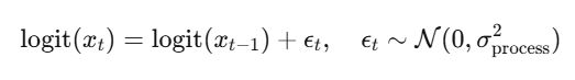
观测结果是对真实状态的 带噪声测量:
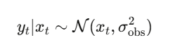
Particle Filter 实时更新概率
粒子滤波维护 N 个概率假设(particles)。每个particles都是关于真实概率的一个假设,并随着数据的到达而重新加权:
1.  INITIALIZE: Draw x_0^{(i)} ~ Prior for i = 1,...,N
    Set weights w_0^{(i)} = 1/N

2.  FOR each new observation y_t:
    a. PROPAGATE:  x_t^{(i)} ~ f( · | x_{t-1}^{(i)} )
    b. REWEIGHT:   w_t^{(i)} ∝ g( y_t | x_t^{(i)} )
    c. NORMALIZE:  w̃_t^{(i)} = w_t^{(i)} / Σ_j w_t^{(j)}
    d. RESAMPLE if ESS = 1/Σ(w̃_t^{(i)})² < N/2
import numpy as np
from scipy.special import expit, logit  # sigmoid and logit

class PredictionMarketParticleFilter:
    """
    Sequential Monte Carlo filter for real-time event probability estimation.

    Usage during a live event (e.g., election night):
        pf = PredictionMarketParticleFilter(prior_prob=0.50)
        pf.update(observed_price=0.55)   # market moves on early returns
        pf.update(observed_price=0.62)   # more data
        pf.update(observed_price=0.58)   # partial correction
        print(pf.estimate())             # filtered probability
    """
    def __init__(self, N_particles=5000, prior_prob=0.5,
                 process_vol=0.05, obs_noise=0.03):
        self.N = N_particles
        self.process_vol = process_vol
        self.obs_noise = obs_noise

        # Initialize particles around prior
        logit_prior = logit(prior_prob)
        self.logit_particles = logit_prior + np.random.normal(0, 0.5, N_particles)
        self.weights = np.ones(N_particles) / N_particles
        self.history = []

    def update(self, observed_price):
        """Incorporate a new observation (market price, poll result, etc.)"""
        # 1. Propagate: random walk in logit space
        noise = np.random.normal(0, self.process_vol, self.N)
        self.logit_particles += noise

        # 2. Convert to probability space
        prob_particles = expit(self.logit_particles)

        # 3. Reweight: likelihood of observation given each particle
        log_likelihood = -0.5 * ((observed_price - prob_particles) / self.obs_noise)**2
        log_weights = np.log(self.weights + 1e-300) + log_likelihood

        # Normalize in log space for stability
        log_weights -= log_weights.max()
        self.weights = np.exp(log_weights)
        self.weights /= self.weights.sum()

        # 4. Check ESS and resample if needed
        ess = 1.0 / np.sum(self.weights**2)
        if ess < self.N / 2:
            self._systematic_resample()

        self.history.append(self.estimate())

    def _systematic_resample(self):
        """Systematic resampling - lower variance than multinomial."""
        cumsum = np.cumsum(self.weights)
        u = (np.arange(self.N) + np.random.uniform()) / self.N
        indices = np.searchsorted(cumsum, u)
        self.logit_particles = self.logit_particles[indices]
        self.weights = np.ones(self.N) / self.N

    def estimate(self):
        """Weighted mean probability estimate."""
        prob_particles = expit(self.logit_particles)
        return np.sum(self.weights * prob_particles)

    def credible_interval(self, alpha=0.05):
        """Weighted quantile-based credible interval."""
为什么不直接使用市场价格?
一个自然的问题是:既然市场价格就是概率,为什么还要过滤?
原因在于,市场价格本身存在 微观噪声。
例如,一笔较大的交易可能让价格从 0.58 → 0.65,但真实概率可能只发生了很小变化。
粒子滤波能够平滑短期噪声、保留信息变化,同时传播不确定性,这正是机构级预测模型的核心能力。
5. 三个常见的方差降低技巧
在Monte Carlo体系中,还有三类经常与前述方法叠加使用的技术。
对称采样
当收益函数是单调的(二元合约价格越高,超过行权价的概率就越高),方差减少就能得到保证:
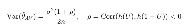
实际效果的减少量通常在50% – 75%。 除了将函数评估次数翻倍(无论如何你都要这样做)之外,无需任何额外的计算成本。
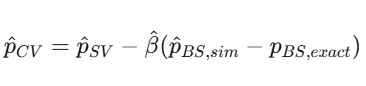
充分利用已有知识
如果你正在模拟随机波动率下的二元合约 ${S_T > K}$(无封闭形式),请使用 Black-Scholes 数字价格 $p_{BS}$(有封闭形式)作为控制变量 :
分而治之
将概率空间划分为多个层,在每个层内进行抽样,然后合并。方差始终 ≤ 粗 MC(根据总方差定律),通过 Neyman 分配可获得最大收益 :$n_j \propto \omega_j \sigma_j$(对方差高的层进行过采样)。
示例代码:
def stratified_binary_mc(S0, K, sigma, T, J=10, N_total=100_000):
    """
    Stratified MC for binary contract pricing.
    Strata defined by quantiles of the terminal price distribution.
    """
    from scipy.stats import norm
    n_per_stratum = N_total // J
    estimates = []

    for j in range(J):
        # Uniform draws within stratum [j/J, (j+1)/J]
        U = np.random.uniform(j/J, (j+1)/J, n_per_stratum)
        Z = norm.ppf(U)
        S_T = S0 * np.exp((-0.5*sigma**2)*T + sigma*np.sqrt(T)*Z)
        stratum_mean = (S_T > K).mean()
        estimates.append(stratum_mean)

    # Each stratum has weight 1/J
    p_stratified = np.mean(estimates)
    se_stratified = np.std(estimates) / np.sqrt(J)

    return p_stratified, se_stratified

p, se = stratified_binary_mc(S0=100, K=105, sigma=0.20, T=30/365)
print(f"Stratified estimate: {p:.6f} ± {se:.6f}")
将上面三个方法堆叠起来
在每个层内引入相反变量,并进行控制变量校正,通常可以实现比原始 MC 值降低 100-500 倍的方差。这在生产中并非可有可无,而是基本要求。
6. 建模相关矩阵无法做到的事情
分层贝叶斯模型通过共享的国家波动参数隐式地编码相关性。
但是尾部依赖性呢 ?尾部依赖性是指极端的共同波动,而这种波动在线性相关性中却无法体现出来。
2008 年,高斯 copula 函数无法有效模拟尾部相关性,这导致了全球金融危机。在预测市场中,也存在同样的问题:当某个摇摆状态出现意外结果时, 所有摇摆状态同时翻转的概率远高于高斯 copula 函数的预测值。
斯克拉定理
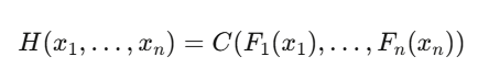
其中 C 是 copula 函数(纯依赖结构),$F_i$ 是边际累积分布函数。您可以分别对每个市场的边际行为进行建模,然后使用 copula 函数将它们连接起来,该 copula 函数能够捕捉包括尾部在内的依赖关系。
尾部依赖问题
高斯 copula :尾部相关性 $\lambda_U = \lambda_L = 0$。极端的协同运动被建模为具有零概率。
对于相关预测市场而言, 这是灾难性的错误。
模拟预测
import numpy as np
from scipy.stats import norm, t as t_dist

def simulate_correlated_outcomes_gaussian(probs, corr_matrix, N=100_000):
    """Gaussian copula no tail dependence."""
    d = len(probs)
    L = np.linalg.cholesky(corr_matrix)
    Z = np.random.standard_normal((N, d))
    X = Z @ L.T
    U = norm.cdf(X)
    outcomes = (U < np.array(probs)).astype(int)
    return outcomes

def simulate_correlated_outcomes_t(probs, corr_matrix, nu=4, N=100_000):
    """Student-t copula symmetric tail dependence."""
    d = len(probs)
    L = np.linalg.cholesky(corr_matrix)
    Z = np.random.standard_normal((N, d))
    X = Z @ L.T

    # Divide by sqrt(chi-squared / nu) to get t-distributed
    S = np.random.chisquare(nu, N) / nu
    T = X / np.sqrt(S[:, None])
    U = t_dist.cdf(T, nu)
    outcomes = (U < np.array(probs)).astype(int)
    return outcomes

def simulate_correlated_outcomes_clayton(probs, theta=2.0, N=100_000):
    """Clayton copula (bivariate) lower tail dependence."""
    # Marshall-Olkin algorithm
    V = np.random.gamma(1/theta, 1, N)
    E = np.random.exponential(1, (N, len(probs)))
    U = (1 + E / V[:, None])**(-1/theta)
    outcomes = (U < np.array(probs)).astype(int)
    return outcomes

# --- Compare tail behavior ---
probs = [0.52, 0.53, 0.51, 0.48, 0.50]  # 5 swing state probabilities
state_names = ['PA', 'MI', 'WI', 'GA', 'AZ']

corr = np.array([
    [1.0, 0.7, 0.7, 0.4, 0.3],
    [0.7, 1.0, 0.8, 0.3, 0.3],
    [0.7, 0.8, 1.0, 0.3, 0.3],
    [0.4, 0.3, 0.3, 1.0, 0.5],
    [0.3, 0.3, 0.3, 0.5, 1.0],
])

N = 500_000

gauss_outcomes = simulate_correlated_outcomes_gaussian(probs, corr, N)
t_outcomes = simulate_correlated_outcomes_t(probs, corr, nu=4, N=N)

# P(sweep all 5 states)
p_sweep_gauss = gauss_outcomes.all(axis=1).mean()
p_sweep_t = t_outcomes.all(axis=1).mean()

# P(lose all 5 states)
p_lose_gauss = (1 - gauss_outcomes).all(axis=1).mean()
p_lose_t = (1 - t_outcomes).all(axis=1).mean()

# If independent
p_sweep_indep = np.prod(probs)
p_lose_indep = np.prod([1-p for p in probs])

print("Joint Outcome Probabilities:")
print(f"{'':>25}  {'Independent':>12}  {'Gaussian':>12}  {'t-copula':>12}")
print(f"{'P(sweep all 5)':>25}  {p_sweep_indep:>12.4f}  {p_sweep_gauss:>12.4f}  {p_sweep_t:>12.4f}")
print(f"{'P(lose all 5)':>25}  {p_lose_indep:>12.4f}  {p_lose_gauss:>12.4f}  {p_lose_t:>12.4f}")
print(f"\nt-copula increases sweep probability by {p_sweep_t/p_sweep_gauss:.1f}x vs Gaussian")
这正是高斯 copula 在 2008 年失败的原因 ,也是它在预测市场组合方面会再次失败的原因。
$\nu = 4$ 的 t-copula 通常显示极端联合结果的概率高出 2-5 倍。
如果你在交易相关预测市场合约时没有对尾部依赖性进行建模,那么你的投资组合就会在最重要的场景中彻底崩盘。
7. 基于代理的仿真
到目前为止,所有步骤都假设您了解数据生成过程,只需要对其进行模拟即可。
但预测市场由各种各样的参与者组成 ——知情交易者、噪音交易者、做市商和机器人,他们的互动产生了涌现的动态,这是任何封闭形式的随机微分方程都无法捕捉的。
零智能启示录
即使每个交易者都完全非理性,市场仍然可以是有效的 。
Gode 和 Sunder (1993) 证明,零智能代理(仅受预算约束而提交随机订单的交易员)在连续双向拍卖中实现了接近 100% 的配置效率。
Farmer、Patelli 和 Zovko (2005) 将此扩展到限制订单簿。
这解释了伦敦证券交易所96%的横截面价差变动。仅一个参数,就占了96%。
基于代理的预测市场模拟器
import numpy as np
from collections import deque

class PredictionMarketABM:
    """
    Agent-based model of a prediction market order book.

    Agent types:
    - Informed: know the true probability, trade toward it
    - Noise: random trades
    - Market maker: provides liquidity around current price
    """
    def __init__(self, true_prob, n_informed=10, n_noise=50, n_mm=5):
        self.true_prob = true_prob
        self.price = 0.50  # initial price
        self.price_history = [self.price]

        # Order book (simplified as bid/ask queues)
        self.best_bid = 0.49
        self.best_ask = 0.51

        # Agent populations
        self.n_informed = n_informed
        self.n_noise = n_noise
        self.n_mm = n_mm

        # Track metrics
        self.volume = 0
        self.informed_pnl = 0
        self.noise_pnl = 0

    def step(self):
        """One time step: randomly select an agent to trade."""
        total = self.n_informed + self.n_noise + self.n_mm
        r = np.random.random()

        if r < self.n_informed / total:
            self._informed_trade()
        elif r < (self.n_informed + self.n_noise) / total:
            self._noise_trade()
        else:
            self._mm_update()

        self.price_history.append(self.price)

    def _informed_trade(self):
        """Informed trader: buy if price < true_prob, sell otherwise."""
        signal = self.true_prob + np.random.normal(0, 0.02)  # noisy signal

        if signal > self.best_ask + 0.01:  # buy
            size = min(0.1, abs(signal - self.price) * 2)
            self.price += size * self._kyle_lambda()
            self.volume += size
            self.informed_pnl += (self.true_prob - self.best_ask) * size
        elif signal < self.best_bid - 0.01:  # sell
            size = min(0.1, abs(self.price - signal) * 2)
            self.price -= size * self._kyle_lambda()
            self.volume += size
            self.informed_pnl += (self.best_bid - self.true_prob) * size

        self.price = np.clip(self.price, 0.01, 0.99)
        self._update_book()

    def _noise_trade(self):
        """Noise trader: random buy/sell."""
        direction = np.random.choice([-1, 1])
        size = np.random.exponential(0.02)
        self.price += direction * size * self._kyle_lambda()
        self.price = np.clip(self.price, 0.01, 0.99)
        self.volume += size
        self.noise_pnl -= abs(self.price - self.true_prob) * size * 0.5
        self._update_book()

    def _mm_update(self):
        """Market maker: tighten spread toward current price."""
        spread = max(0.02, 0.05 * (1 - self.volume / 100))
        self.best_bid = self.price - spread / 2
        self.best_ask = self.price + spread / 2

    def _kyle_lambda(self):
        """Price impact parameter."""
        sigma_v = abs(self.true_prob - self.price) + 0.05
        sigma_u = 0.1 * np.sqrt(self.n_noise)
        return sigma_v / (2 * sigma_u)

    def _update_book(self):
        spread = self.best_ask - self.best_bid
        self.best_bid = self.price - spread / 2
        self.best_ask = self.price + spread / 2

    def run(self, n_steps=1000):
        for _ in range(n_steps):
            self.step()
        return np.array(self.price_history)

# --- Simulation ---
np.random.seed(42)

# Scenario: true probability is 0.65, market starts at 0.50
sim = PredictionMarketABM(true_prob=0.65, n_informed=10, n_noise=50, n_mm=5)
prices = sim.run(n_steps=2000)

print("Agent-Based Prediction Market Simulation")
print(f"True probability:   {sim.true_prob:.2f}")
print(f"Starting price:     0.50")
print(f"Final price:        {prices[-1]:.4f}")
print(f"Price at t=500:     {prices[500]:.4f}")
print(f"Price at t=1000:    {prices[1000]:.4f}")
print(f"Total volume:       {sim.volume:.1f}")
print(f"Informed P&L:       ${sim.informed_pnl:.2f}")
print(f"Noise trader P&L:   ${sim.noise_pnl:.2f}")
print(f"Convergence error:  {abs(prices[-1] - sim.true_prob):.4f}")
价格收敛的速度取决于知情交易者与噪音交易者的比例、做市商价差对信息流的反应,以及知情交易者为何以噪音交易者的损失为代价来获取利润。
8. 生产堆栈
一个完整的机构级模拟系统可以划分为五个核心层级:
第一层:数据采集层
通过 WebSocket 获取 Polymarket 等平台的 CLOB 实时价格,并利用 NLP 技术将新闻和民调转化为概率信号。
第二层:概率引擎层
基于 Stan 或 PyMC 的层次贝叶斯模型生成后验分布,并结合粒子滤波器进行实时更新,通过跳跃扩散过程(Jump-diffusion)模拟路径风险。
第三层:依赖建模层
使用藤 Copula 处理合约间的成对依赖,并通过因子模型剥离国家级或全球性的系统风险因素。
第四层:风险管理层
基于极值理论(EVT)计算 VaR 和期望损失(Expected Shortfall),进行压力测试以识别最坏情境,并严密监控订单簿深度以应对流动性风险。
第五层:监控归因层
持续追踪 Brier Score 以确保模型定标未失效,并进行损益归因(P&L Attribution),明确各模型组件的贡献度。
在当前的预测市场中,如果不具备模拟尾部相关性和实时过滤噪声的能力,所持有的组合在关键时刻将面临巨大的崩塌风险。
总结
回顾整个路径,可以看到一个逐层升级的模拟体系:
最开始只是一个简单问题:
“事件概率是多少?”
但随着模型不断深化,系统逐渐扩展为:
- 蒙特卡洛 概率估计
- Importance Sampling 尾部风险
- Sequential Monte Carlo 实时更新
- 多层方差控制技术
最终形成的,是量化交易台使用的 概率模拟引擎。
抛硬币模型只有一个参数。
真实市场的概率系统,却包含整个动态世界。
而理解这条路径,是进入 机构级量化研究 的第一步。如果你想了解更多关于Python在量化领域的实战应用,欢迎在云栈社区与同行交流探讨。
 发表于 2026-3-7 16:42:47
|
查看: 317|
回复: 0
发表于 2026-3-7 16:42:47
|
查看: 317|
回复: 0
