数据增强理论与实践：从VRM、Mixup到PyTorch图像分类实战

数据增强是一种通过人工引入扰动来扩充训练数据多样性的强大技术。它的理论基础可以从风险最小化、近域风险最小化（Vicinal Risk Minimization, VRM）、群不变性、噪声注入与正则化的联系，以及Mixup、CutMix等具体方法的数学推理等多个角度来理解。

从经验风险到增广的经验风险

设监督学习问题的输入空间为 $\mathcal{X}$，标签空间为 $\mathcal{Y}$，样本从未知分布 $P(x, y)$ 中抽取。我们有训练集 $S = \{(x_i, y_i)\}_{i=1}^n$，目标是学习一个函数 $f_\theta$（以参数 $\theta$ 表示）以最小化期望风险：

由于 $P$ 未知，通常采用经验风险最小化（ERM）：

数据增强引入一个变换算子 $T(\cdot; \epsilon)$，其中 $\epsilon$ 是变换参数（如旋转角度、平移距离等），并假定 $\epsilon$ 由某已知分布 $p(\epsilon)$ 采样。
增强过程可理解为在训练中对每个样本应用随机变换：

其中 $y_i(\epsilon)$ 为增强后对应的标签。对于保持语义不变的增强（如几何、颜色变换），通常 $y_i(\epsilon) = y_i$；对于Mixup、CutMix等特殊增强，标签为软组合。

于是增广的经验风险定义为：

训练时我们用蒙特卡洛近似该期望，对每个样本独立采样 $\epsilon_i \sim p(\epsilon)$，得到无偏估计：

若 $f_\theta$ 可微且每次更新使用该无偏采样，则梯度的期望同样是无偏的：

这意味着单步随机增强梯度是对真实增广风险梯度的无偏估计。此外，重复采样次数 $M$（对同一样本进行 $M$ 次增强）越大，方差越小，但计算开销也越大。在实践中通常 $M=1$ 或小值即可。

VRM 与数据增强的理论框架

近域风险最小化（VRM）由Chapelle等人提出，其核心思想是在训练样本附近构造邻域分布，以近似原始未知分布，从而改善模型泛化能力。
设邻域分布定义为：

其中 $\nu(x|x_i)$ 是围绕 $x_i$ 的密度（如加性噪声、局部仿射变换、颜色抖动等），$\delta$ 为Dirac delta函数（标签保持不变）。VRM的经验风险为：

将 $\nu(x|x_i)$ 替换为数据增强诱导的分布 $p(T(x_i; \epsilon))$，即可得到与上一节一致的公式。直观地，VRM通过填充训练样本周围的概率质量，促使模型在局部邻域具有平滑性、不变性或等变性，从而提升泛化能力。

当增强变换来自某个变换群（如旋转群、平移群），且任务本身对该变换具有不变性（如图像分类对轻微平移、旋转不敏感）时，随机采样 $\epsilon$ 并作用于输入，等价于近似训练一个对该变换群不变或等变的模型。这种群增强可看作对数据分布进行群平均：

其中 $\mu$ 为群 $G$ 上的概率测度（如均匀分布）。若模型 $f_\theta$ 满足某种等变性，则可以证明在某些条件下，最小化增广风险可促使模型输出在群作用下的具有一致性或稳定性，这对于减少过拟合、提高模型鲁棒性有显著作用。

噪声注入与正则化的联系

以线性模型 $f_\theta(x) = \theta^T x$ 与平方损失 $\mathcal{L}(\hat{y}， y) = (\hat{y} - y)^2$ 为例。
对输入施加加性高斯噪声 $T(x; \epsilon) = x + \epsilon$，其中 $\epsilon \sim \mathcal{N}(0， \sigma^2 I)$。
增强后的期望损失为：

这表明对输入加入高斯噪声对线性回归的效果等价于在损失函数中加入 $\ell_2$ 正则项（Tikhonov正则化），其强度与噪声方差 $\sigma^2$ 成正比。

Mixup 与 CutMix

Mixup：从两个样本 $(x_i， y_i)$ 与 $(x_j， y_j)$ 构建线性插值样本：

其中 $\lambda \sim \text{Beta}(\alpha， \alpha)$，常用 $\alpha \in [0.1， 0.4]$。对于分类任务，$y_i$， $y_j$ 通常为one-hot向量，所得 $\tilde{y}$ 为软标签。Mixup的损失（交叉熵）为：

其梯度为：

等价于对两类的交叉熵梯度进行加权平均。
因此，Mixup鼓励模型在输入空间的线性路径上输出也呈线性变化，强化了决策边界的平滑性与大间隔特性，有效减少对单个训练点的过拟合。

CutMix：在图像空间进行矩形区域裁剪与粘贴，将 $x_j$ 的一块区域粘贴到 $x_i$ 上，并按面积比例调整标签：

其中 $M$ 为二值掩膜（1表示保留 $x_i$ 的区域，0表示替换为 $x_j$ 的区域），$\lambda$ 为掩膜中1所占的面积比。CutMix在保留图像局部结构的同时进行类别信息的局部混合，能提升模型对遮挡、局部噪声的鲁棒性，并通过标签软分配抑制过拟合。

Mixup与CutMix可归入VRM框架中的邻域分布构造，但其邻域不再是对单个样本的局部扰动，而是对两个样本的凸组合或局部拼接。其理论动机是扩大训练分布的支撑（support），让模型在更广阔的输入空间形成更平滑、更稳健的决策边界。

常见增强方法分类与数学化描述

• 几何类增强（假定标签不变）：

  • 旋转：$T(x; \theta) = R_\theta x$
  • 平移：$T(x; \Delta x， \Delta y) = \text{Translate}(x， (\Delta x， \Delta y))$
  • 缩放：$T(x; s) = \text{Scale}(x， s)$
  • 透视变换：$T(x; \text{persp_params}) = \text{Perspective}(x， \text{persp_params})$

• 颜色增强（标签通常不变，但要注意任务敏感性）：

  • 亮度、对比度、饱和度、色相抖动：$T(x; \beta， \gamma， \eta， \phi) = \text{Jitter}(x， \beta， \gamma， \eta， \phi)$

• 噪声/模糊增强：

  • 高斯噪声：$T(x; \epsilon) = x + \epsilon， \quad \epsilon \sim \mathcal{N}(0， \sigma^2 I)$
  • 模糊卷积：$T(x; k) = \text{Blur}(x， k)$

• 随机擦除/遮挡：

  • Cutout/Random Erasing：$T(x; M) = M \odot x$

• 标签软分配增强：

  • Mixup：见上文
  • CutMix：见上文

这些方法可以组合使用，形成多步增强流水线。一条增强管线的总体分布是各步骤参数分布的联合。

完整实战案例：基于PyTorch的图像分类增强实验

我们构造一个多类合成图像数据集，每张图为64x64彩色图像，包含三类：

• 类A：红色圆形
• 类B：蓝色方形
• 类C：绿色三角形
  背景存在轻微噪声，并模拟类别数量不完全平衡的情况。我们使用以下增强组合：
  1. 几何：随机仿射（旋转、平移、缩放、剪切）、随机透视、随机水平翻转
  2. 颜色：亮度/对比度/饱和度/色相抖动
  3. 噪声：加性高斯噪声
  4. 遮挡：Random Erasing
  5. 标签软增强：Mixup（Beta分布）与CutMix（随机矩形）

随后，我们训练一个小型卷积神经网络（CNN）并在验证集上进行可视化与评估。

import os
import random
import math
import numpy as np
from PIL import Image, ImageDraw
import matplotlib.pyplot as plt
from matplotlib.colors import ListedColormap
import seaborn as sns
import torch
import torch.nn as nn
import torch.nn.functional as F
import torchvision.transforms as transforms
from torch.utils.data import Dataset, DataLoader
from sklearn.manifold import TSNE
from sklearn.metrics import confusion_matrix

# 1) 设置随机种子保证可复现性
def set_seed(seed=42):
    random.seed(seed)
    np.random.seed(seed)
    torch.manual_seed(seed)
    torch.backends.cudnn.benchmark = False
    torch.backends.cudnn.deterministic = True
set_seed(1234)
device = torch.device("cuda" if torch.cuda.is_available() else "cpu")

# 2) 合成数据集：几何图形
class SyntheticShapesDataset(Dataset):
    def __init__(self, n_samples=600, image_size=64, split='train',
                 class_probs=(0.34, 0.33, 0.33), transform=None):
        self.n_samples = n_samples
        self.image_size = image_size
        self.split = split
        self.transform = transform
        self.class_probs = class_probs  # 模拟不平衡
        self.data = []
        self.labels = []
        self._generate()
    def _generate(self):
        H = W = self.image_size
        for i in range(self.n_samples):
            cls = np.random.choice([0,1,2], p=self.class_probs)
            img = (np.random.rand(H, W, 3) * 25).astype(np.uint8)  # 暗背景带噪声
            img = Image.fromarray(img, mode='RGB')
            draw = ImageDraw.Draw(img)
            min_size = int(self.image_size * 0.25)
            max_size = int(self.image_size * 0.55)
            size = np.random.randint(min_size, max_size)
            cx = np.random.randint(size//2 + 2, W - size//2 - 2)
            cy = np.random.randint(size//2 + 2, H - size//2 - 2)
            if cls == 0:
                color = (255, 0, 0)
                bbox = [cx - size//2, cy - size//2, cx + size//2, cy + size//2]
                draw.ellipse(bbox, fill=color, outline=(255, 255, 255))
            elif cls == 1:
                color = (0, 0, 255)
                bbox = [cx - size//2, cy - size//2, cx + size//2, cy + size//2]
                draw.rectangle(bbox, fill=color, outline=(255, 255, 255))
            else:
                color = (0, 255, 0)
                half = size//2
                p1 = (cx, cy - half)
                p2 = (cx - half, cy + half)
                p3 = (cx + half, cy + half)
                draw.polygon([p1, p2, p3], fill=color, outline=(255, 255, 255))
            self.data.append(img)
            self.labels.append(cls)
    def __len__(self):
        return self.n_samples
    def __getitem__(self, idx):
        img = self.data[idx]
        y = self.labels[idx]
        if self.transform is not None:
            img = self.transform(img)
        return img, y

# 3) 自定义增强类（记录参数分布用于分析）
class LogRandomAffine(transforms.RandomAffine):
    def __init__(self, degrees, translate=None, scale=None, shear=None):
        super().__init__(degrees=degrees, translate=translate, scale=scale, shear=shear)
        self.log = {"angle": [], "translate_x": [], "translate_y": [],
                    "scale": [], "shear": []}
    def get_params(self, degrees, translate, scale_ranges, shears, img_size):
        params = super().get_params(degrees, translate, scale_ranges, shears, img_size)
        angle, translations, scale, shear = params
        self.log["angle"].append(angle)
        self.log["translate_x"].append(translations[0])
        self.log["translate_y"].append(translations[1])
        self.log["scale"].append(scale if scale is not None else 1.0)
        self.log["shear"].append(shear[0] if isinstance(shear, (list, tuple)) else (shear if shear is not None else 0.0))
        return params
class LogRandomPerspective(transforms.RandomPerspective):
    def __init__(self, distortion_scale=0.5, p=0.5, interpolation=Image.BILINEAR):
        super().__init__(distortion_scale=distortion_scale, p=p, interpolation=interpolation)
        self.log = {"distortion_scale": []}
    def get_params(self, width, height, distortion_scale):
        startpoints, endpoints = super().get_params(width, height, distortion_scale)
        self.log["distortion_scale"].append(distortion_scale)
        return startpoints, endpoints
class LogColorJitter(transforms.ColorJitter):
    def __init__(self, brightness=0.4, contrast=0.4, saturation=0.4, hue=0.1):
        super().__init__(brightness=brightness, contrast=contrast, saturation=saturation, hue=hue)
        self.log = {"brightness": [], "contrast": [], "saturation": [], "hue": []}
    def get_params(self, brightness, contrast, saturation, hue):
        fn_idx, b, c, s, h = super().get_params(brightness, contrast, saturation, hue)
        self.log["brightness"].append(0 if b is None else b)
        self.log["contrast"].append(0 if c is None else c)
        self.log["saturation"].append(0 if s is None else s)
        self.log["hue"].append(0 if h is None else h)
        return fn_idx, b, c, s, h
class AddGaussianNoise(nn.Module):
    def __init__(self, mean=0.0, std=0.02):
        super().__init__()
        self.mean = mean
        self.std = std
        self.log = {"std": []}
    def forward(self, tensor):
        noise = torch.randn_like(tensor) * self.std + self.mean
        self.log["std"].append(self.std)
        return tensor + noise

# 4) Mixup 与 CutMix 实现
def one_hot(labels, num_classes):
    return F.one_hot(torch.as_tensor(labels, dtype=torch.long), num_classes=num_classes).float()
def mixup_data(x, y, alpha=0.4):
    lam = np.random.beta(alpha, alpha) if alpha > 0 else 1.0
    batch_size = x.size()[0]
    index = torch.randperm(batch_size).to(x.device)
    mixed_x = lam * x + (1 - lam) * x[index, :]
    y_a, y_b = y, y[index]
    lam_tensor = torch.tensor(lam, dtype=torch.float, device=x.device)
    return mixed_x, y_a, y_b, lam_tensor
def cutmix_data(x, y, alpha=0.7):
    lam = np.random.beta(alpha, alpha) if alpha > 0 else 1.0
    batch_size, _, H, W = x.size()
    index = torch.randperm(batch_size).to(x.device)
    cut_rat = np.sqrt(1. - lam)
    cut_w = int(W * cut_rat)
    cut_h = int(H * cut_rat)
    cx = np.random.randint(W)
    cy = np.random.randint(H)
    x1 = np.clip(cx - cut_w // 2, 0, W)
    y1 = np.clip(cy - cut_h // 2, 0, H)
    x2 = np.clip(cx + cut_w // 2, 0, W)
    y2 = np.clip(cy + cut_h // 2, 0, H)
    x_clone = x.clone()
    x_clone[:, :, y1:y2, x1:x2] = x[index, :, y1:y2, x1:x2]
    lam_adjusted = 1.0 - ((x2 - x1) * (y2 - y1) / (W * H))
    lam_tensor = torch.tensor(lam_adjusted, dtype=torch.float, device=x.device)
    y_a, y_b = y, y[index]
    return x_clone, y_a, y_b, lam_tensor
def soft_target_cross_entropy(logits, targets):
    log_probs = F.log_softmax(logits, dim=1)
    loss = -(targets * log_probs).sum(dim=1).mean()
    return loss

# 5) 简单CNN模型定义
class SimpleCNN(nn.Module):
    def __init__(self, num_classes=3):
        super().__init__()
        self.conv1 = nn.Conv2d(3, 32, kernel_size=3, padding=1)
        self.bn1 = nn.BatchNorm2d(32)
        self.conv2 = nn.Conv2d(32, 64, kernel_size=3, padding=1)
        self.bn2 = nn.BatchNorm2d(64)
        self.conv3 = nn.Conv2d(64, 128, kernel_size=3, padding=1)
        self.bn3 = nn.BatchNorm2d(128)
        self.pool = nn.MaxPool2d(2)
        self.dropout = nn.Dropout(0.25)
        self.fc1 = nn.Linear(128 * 8 * 8, 256)
        self.fc2 = nn.Linear(256, num_classes)
    def forward(self, x, return_features=False):
        x = self.pool(F.relu(self.bn1(self.conv1(x))))
        x = self.pool(F.relu(self.bn2(self.conv2(x))))
        x = self.pool(F.relu(self.bn3(self.conv3(x))))
        x = x.view(x.size(0), -1)
        feat = F.relu(self.fc1(x))
        feat = self.dropout(feat)
        logits = self.fc2(feat)
        if return_features:
            return logits, feat
        return logits

# 6) 定义增强管线（带参数日志）
affine = LogRandomAffine(degrees=30, translate=(0.1,0.1), scale=(0.8,1.2), shear=10)
perspective = LogRandomPerspective(distortion_scale=0.5, p=0.3)
jitter = LogColorJitter(brightness=0.4, contrast=0.4, saturation=0.4, hue=0.1)
gaussian_noise = AddGaussianNoise(mean=0.0, std=0.02)
train_transform = transforms.Compose([
    affine,
    transforms.RandomHorizontalFlip(p=0.5),
    perspective,
    jitter,
    transforms.ToTensor(),
    gaussian_noise,
    transforms.RandomErasing(p=0.4, scale=(0.02, 0.2), ratio=(0.3, 3.3))
])
test_transform = transforms.Compose([
    transforms.ToTensor()
])

# 7) 构造数据集与数据加载器
train_set = SyntheticShapesDataset(n_samples=720, image_size=64, split='train',
                                 class_probs=(0.36, 0.32, 0.32), transform=train_transform)
val_set = SyntheticShapesDataset(n_samples=240, image_size=64, split='val',
                               class_probs=(0.34, 0.33, 0.33), transform=test_transform)
train_loader = DataLoader(train_set, batch_size=64, shuffle=True, num_workers=0)
val_loader = DataLoader(val_set, batch_size=64, shuffle=False, num_workers=0)

# 8) 训练循环（含Mixup/CutMix）
model = SimpleCNN(num_classes=3).to(device)
optimizer = torch.optim.Adam(model.parameters(), lr=1e-3)
scheduler = torch.optim.lr_scheduler.StepLR(optimizer, step_size=6, gamma=0.6)
num_epochs = 12
mixup_alpha = 0.4
cutmix_alpha = 0.7
prob_mixup = 0.5
prob_cutmix = 0.3
train_losses, val_losses = [], []
train_accs, val_accs = [], []
mix_lam_log = []
cutmix_lam_log = []
def accuracy_from_logits(logits, labels):
    preds = logits.argmax(dim=1)
    return (preds == labels).float().mean().item()
for epoch in range(1, num_epochs+1):
    model.train()
    running_loss, running_acc, n_total = 0.0, 0.0, 0
    for x, y in train_loader:
        x, y = x.to(device), y.to(device)
        rnd = np.random.rand()
        use_mixup = rnd < prob_mixup
        use_cutmix = (rnd >= prob_mixup) and (rnd < (prob_mixup + prob_cutmix))
        optimizer.zero_grad()
        if use_mixup:
            x_mixed, y_a, y_b, lam = mixup_data(x, y, alpha=mixup_alpha)
            logits = model(x_mixed)
            ya_oh = one_hot(y_a, num_classes=3).to(device)
            yb_oh = one_hot(y_b, num_classes=3).to(device)
            targets = lam * ya_oh + (1-lam) * yb_oh
            loss = soft_target_cross_entropy(logits, targets)
            mix_lam_log.append(lam.item())
            acc = accuracy_from_logits(logits, y_a)  # 近似参考
        elif use_cutmix:
            x_cm, y_a, y_b, lam = cutmix_data(x, y, alpha=cutmix_alpha)
            logits = model(x_cm)
            ya_oh = one_hot(y_a, num_classes=3).to(device)
            yb_oh = one_hot(y_b, num_classes=3).to(device)
            targets = lam * ya_oh + (1-lam) * yb_oh
            loss = soft_target_cross_entropy(logits, targets)
            cutmix_lam_log.append(lam.item())
            acc = accuracy_from_logits(logits, y_a)
        else:
            logits = model(x)
            loss = F.cross_entropy(logits, y)
            acc = accuracy_from_logits(logits, y)
        loss.backward()
        optimizer.step()
        batch_size = x.size(0)
        running_loss += loss.item() * batch_size
        running_acc += acc * batch_size
        n_total += batch_size
    train_losses.append(running_loss / n_total)
    train_accs.append(running_acc / n_total)
    # 验证阶段
    model.eval()
    val_running_loss, val_running_acc, val_total = 0.0, 0.0, 0
    all_val_logits, all_val_labels = [], []
    with torch.no_grad():
        for x, y in val_loader:
            x, y = x.to(device), y.to(device)
            logits = model(x)
            loss = F.cross_entropy(logits, y)
            val_running_loss += loss.item() * x.size(0)
            val_running_acc += accuracy_from_logits(logits, y) * x.size(0)
            val_total += x.size(0)
            all_val_logits.append(logits.cpu())
            all_val_labels.append(y.cpu())
    val_losses.append(val_running_loss / val_total)
    val_accs.append(val_running_acc / val_total)
    scheduler.step()
    print(f"Epoch {epoch:02d}/{num_epochs} | Train Loss: {train_losses[-1]:.4f} Acc: {train_accs[-1]:.4f} | Val Loss: {val_losses[-1]:.4f} Acc: {val_accs[-1]:.4f}")

# 9) 验证集特征提取与可视化
model.eval()
val_features, val_labels, val_preds = [], [], []
with torch.no_grad():
    for x, y in val_loader:
        x, y = x.to(device), y.to(device)
        logits, feat = model(x, return_features=True)
        val_features.append(feat.cpu().numpy())
        val_labels.append(y.cpu().numpy())
        val_preds.append(logits.argmax(dim=1).cpu().numpy())
val_features = np.concatenate(val_features, axis=0)
val_labels = np.concatenate(val_labels, axis=0)
val_preds = np.concatenate(val_preds, axis=0)
# t-SNE降维
tsne = TSNE(n_components=2, init='random', random_state=1234, perplexity=30, n_iter=800)
val_tsne = tsne.fit_transform(val_features)
# 混淆矩阵
cm = confusion_matrix(val_labels, val_preds, labels=[0,1,2])

# 10) 绘制分析总图
plt.figure(figsize=(14, 10))
plt.suptitle("数据增强分析总图", fontsize=16, color='darkmagenta')
# 子图1：t-SNE嵌入散点图
ax1 = plt.subplot(2, 2, 1)
colors, markers = ['red', 'blue', 'green'], ['o', 's', '^']
for cls in [0,1,2]:
    idx = (val_labels == cls)
    ax1.scatter(val_tsne[idx, 0], val_tsne[idx, 1], c=colors[cls], s=24,
                marker=markers[cls], alpha=0.85, label=f"Class {cls}")
ax1.set_title("t-SNE验证特征嵌入", color='purple')
ax1.set_xlabel("TSNE-1", color='purple'); ax1.set_ylabel("TSNE-2", color='purple')
ax1.legend(loc='best', fontsize=9); ax1.grid(True, alpha=0.3)
# 子图2：训练/验证曲线
ax2 = plt.subplot(2, 2, 2)
epochs = np.arange(1, num_epochs+1)
ax2.plot(epochs, train_losses, color='magenta', lw=2, label='Train Loss')
ax2.plot(epochs, val_losses, color='orange', lw=2, label='Val Loss')
ax22 = ax2.twinx()
ax22.plot(epochs, train_accs, color='cyan', lw=2, label='Train Acc')
ax22.plot(epochs, val_accs, color='lime', lw=2, label='Val Acc')
ax2.set_title("训练/验证损失与准确率", color='purple')
ax2.set_xlabel("Epoch", color='purple'); ax2.set_ylabel("Loss", color='magenta')
ax22.set_ylabel("Accuracy", color='lime')
lns = ax2.get_lines() + ax22.get_lines(); labs = [l.get_label() for l in lns]
ax2.legend(lns, labs, loc='lower right', fontsize=9); ax2.grid(True, alpha=0.3)
# 子图3：混淆矩阵热力图
ax3 = plt.subplot(2, 2, 3)
sns.heatmap(cm, annot=True, fmt='d', cmap='YlOrRd', cbar=True, ax=ax3)
ax3.set_title("验证集混淆矩阵", color='purple')
ax3.set_xlabel("Predicted", color='purple'); ax3.set_ylabel("True", color='purple')
ax3.set_xticklabels(['Red-Circle','Blue-Square','Green-Triangle'], rotation=30)
ax3.set_yticklabels(['Red-Circle','Blue-Square','Green-Triangle'], rotation=30)
# 子图4：增强参数分布直方图
ax4 = plt.subplot(2, 2, 4)
angles = np.array(affine.log["angle"])
scales = np.array(affine.log["scale"])
pers_scales = np.array(perspective.log["distortion_scale"])
mix_lam = np.array(mix_lam_log) if len(mix_lam_log)>0 else np.array([0.0])
cut_lam = np.array(cutmix_lam_log) if len(cutmix_lam_log)>0 else np.array([0.0])
bins = 20
ax4.hist(angles, bins=bins, alpha=0.7, color='hotpink', label='Affine Angle')
ax4.hist(scales, bins=bins, alpha=0.7, color='deepskyblue', label='Affine Scale')
ax4.hist(pers_scales, bins=bins, alpha=0.7, color='gold', label='Perspective')
ax4.hist(mix_lam, bins=bins, alpha=0.7, color='lime', label='Mixup λ')
ax4.hist(cut_lam, bins=bins, alpha=0.7, color='purple', label='CutMix λ')
ax4.set_title("增强参数分布", color='purple')
ax4.set_xlabel("Value", color='purple'); ax4.set_ylabel("Frequency", color='purple')
ax4.legend(loc='upper right', fontsize=9); ax4.grid(True, alpha=0.3)
plt.tight_layout(rect=[0, 0.03, 1, 0.95])
plt.show()

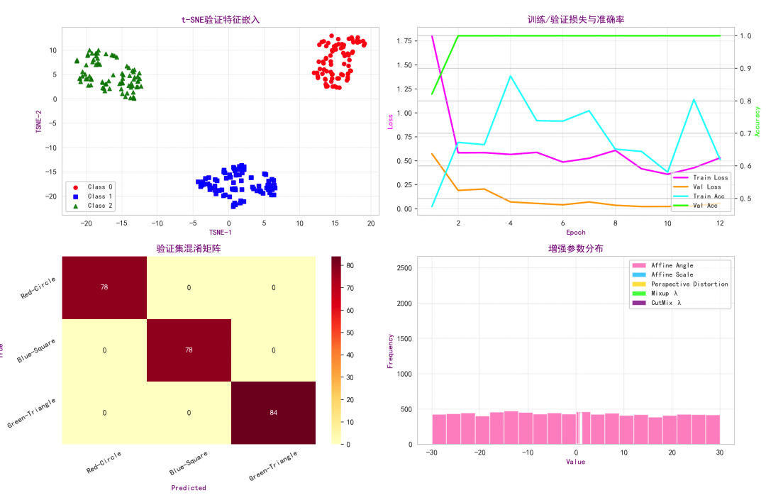
可视化结果分析：

1. t-SNE验证特征嵌入：展示模型在验证集上的特征可分性。若不同类别点（红、蓝、绿）在二维嵌入中形成明显簇且分离良好，说明模型学习到了有判别力的特征。若出现类簇重叠，可能意味着增强过强导致分布漂移、模型容量不足或类间区分度不充分，可通过调节增强强度、增加模型容量或延长训练来解决。

2. 训练/验证损失与准确率曲线：反映训练过程的稳定性与过拟合情况。若训练损失快速下降但验证损失不降或反升，可能说明过拟合；数据增强通常能缓解此现象。若两条曲线较为接近，说明增强带来了良好的正则化效果。曲线波动过大可能需要调节学习率。

3. 混淆矩阵热力图：提供类级别的性能诊断，观察哪些类别之间容易混淆。例如，若绿色三角与蓝色方形混淆较多，可能与几何增强导致形状近似有关，可针对性调整增强策略或检查类别不平衡问题。

4. 增强参数分布：审计训练期间实际采样的增强参数范围与频率，确保增强覆盖了预期的扰动空间。若某些参数（如旋转角度）采样过于集中，可能是配置不当，需检查增强管线的配置与采样策略。Mixup/CutMix的λ分布反映了软标签的插值强度，应避免过度集中在极端值（0或1）附近。

总结

通过VRM的视角，可以将数据增强理解为对训练数据分布的邻域扩展；通过群不变性理论，可将其视为对模型施加的结构性约束；噪声注入的分析则揭示了其与经典正则化方法的联系；而对Mixup、CutMix等方法的解析，展示了通过样本混合来扩大分布支撑、平滑决策边界的思想。

在实践中，基于PyTorch等框架进行数据增强调参的关键在于：

1. 确认任务的不变性与所选增强空间的一致性。
2. 精细调节各类增强的强度与使用概率，避免模型被过度扰动或欠扰动。
3. 对Mixup、CutMix等软标签方法，合理选择Beta分布的参数（α）与混合策略。
4. 充分利用t-SNE、损失曲线、混淆矩阵及参数分布图等可视化工具进行迭代审计与优化。