说明:本文计算量很大、步骤较多,难免存在疏漏,欢迎指正。文中每个计算环节使用的函数均已给出,便于自行修改。本文仅代表个人观点,与任职机构无关。
每当看到代码里出现 “Low Latency” 这类字眼,很多人会下意识把关注点放到“降低静态延迟、扩大带宽、上大规模 ScaleUP 网络”上。但事实真的是这样吗?
本文作为第一篇,先分析 H800 和 H20 在 DeepSeek-R1 的 EP 并行推理性能峰值;后续会继续分析 B200-NVL72 这类实例,看看 ScaleUP 网络是否真的有优势。
TL;DR
H800 和 H20 的分析结果如下(H800 基本能和 DeepSeek 官方数据对齐)。
Prefill 阶段
|
H800 |
H20 |
| TPS(Overlap) |
52240.1 |
9377.0 |
| TPS |
33741.0 |
8536.9 |
Decoding 阶段
|
H800(TP1) |
H800(TP1) |
H800(TP1) |
H20(TP4) |
H20_3e(TP8) |
H20_3e(TP8) |
| BatchSize |
32.000 |
64.000 |
128.000 |
32.000 |
32.000 |
64.000 |
| TPOT(Overlap) |
9.858 |
19.716 |
39.431 |
35.367 |
29.613 |
49.005 |
| TPOT |
17.023 |
34.045 |
68.090 |
42.532 |
36.778 |
63.334 |
| TPS(Overlap) |
101.442 |
50.721 |
25.360 |
28.275 |
33.768 |
20.406 |
| TPS |
58.746 |
29.373 |
14.686 |
23.512 |
27.190 |
15.789 |
| Total(Overlap) |
3246.137 |
3246.137 |
3246.137 |
904.803 |
1080.591 |
1306.001 |
| Total |
1879.856 |
1879.856 |
1879.856 |
752.383 |
870.082 |
1010.516 |
其中 H20-3E(HBM3e-141GB) 在 Decoding 阶段相对于 H20 有接近 1.4x 的性能收益。
本文目录
1. DeepSeek-V3/R1模型架构及计算复杂度分析
1.1 MLA计算复杂度
1.1.1 标准模式
1.1.2 矩阵吸收模式
1.2 DenseMLP计算复杂度
1.3 MoE Expert计算复杂度
1.4 数据汇总
2. Prefill阶段
2.1 MLA计算耗时
2.2 DenseMLP计算耗时
2.3 MoE计算耗时
2.4 AlltoAll通信耗时
2.5 总耗时
2.6 Overlap分析
2.7 KVCache计算
3. Decoding阶段
3.1 EP策略分析
3.2 Memory利用率分析
3.3 MLA耗时
3.4 DenseMLP耗时
3.5 AlltoAll通信耗时
3.6 总耗时
3.7 Overlap分析
4. 小结
1. DeepSeek-V3/R1 模型架构及计算复杂度分析
DeepSeek-V3/R1 模型架构如下:
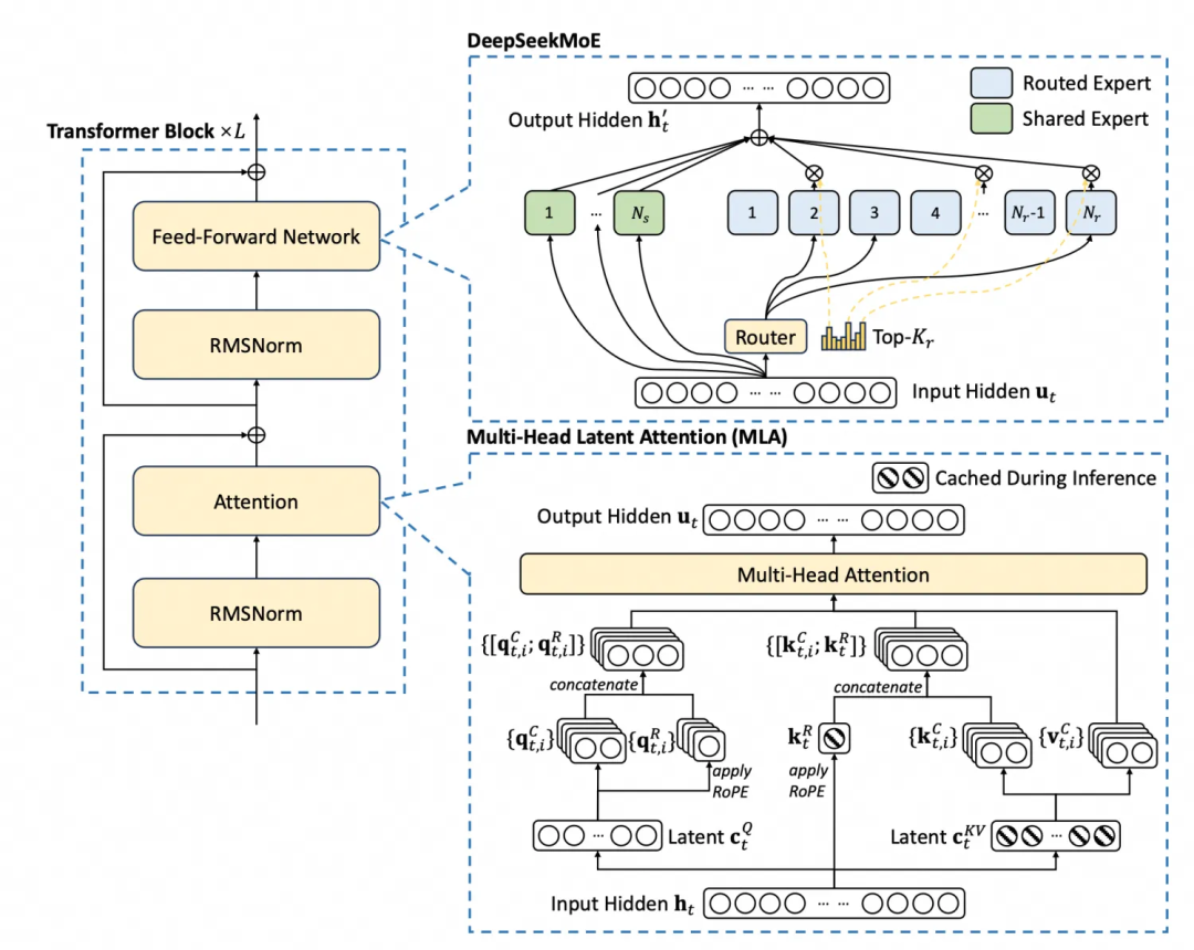
模型参数定义如下:
class ModelArgs:
    max_batch_size: int = 8
    max_seq_len: int = 4096 * 4
    vocab_size: int = 129280
    dim: int = 7168
    inter_dim: int = 18432
    moe_inter_dim: int = 2048
    n_layers: int = 61
    n_dense_layers: int = 3
    n_heads: int = 128
# moe
    n_routed_experts: int = 256
    n_shared_experts: int = 1
    n_activated_experts: int = 8
    n_expert_groups: int = 8
    n_limited_groups: int = 4
    route_scale: float = 2.5
# mla
    q_lora_rank: int = 1536
    kv_lora_rank: int = 512
    qk_nope_head_dim: int = 128
    qk_rope_head_dim: int = 64
    v_head_dim: int = 128
虽然各模块的浮点运算量、参数量有一种很省事的方法:用 ptflops 的 get_model_complexity_info 直接处理 block 得出。但该库对某些复杂算子会统计有误,因此本文对关键部分做了手工校正。
若你对推理系统/模型结构更感兴趣,可以在 人工智能 板块找到更多相关讨论。
1.1 MLA 计算复杂度
1.1.1 标准实现
MLA 模块代码来自 DeepSeek-V3 GitHub 示例,是一个标准 MLA 实现:
class MLA(nn.Module):
def __init__(self, args: ModelArgs):
        super().__init__()
        self.dim = args.dim #隐藏层维度
        self.n_heads = args.n_heads
        self.n_local_heads = args.n_heads // world_size
        self.q_lora_rank = args.q_lora_rank #q的低秩压缩的维度
        self.kv_lora_rank = args.kv_lora_rank #kv的低秩压缩的维度
        self.qk_nope_head_dim = args.qk_nope_head_dim #qk不带旋转位置编码的头的维度
        self.qk_rope_head_dim = args.qk_rope_head_dim #qk旋转位置编码的头的维度
        self.qk_head_dim = args.qk_nope_head_dim + args.qk_rope_head_dim
        self.v_head_dim = args.v_head_dim #v的多头注意力中头的维度

        self.wq_a = nn.Linear(self.dim, self.q_lora_rank)
#q的down-projection矩阵

        self.q_norm = nn.RMSNorm(self.q_lora_rank)

        self.wq_b = nn.Linear(self.q_lora_rank, self.n_heads * self.qk_head_dim)
#q的up-projection矩阵

        self.wkv_a = nn.Linear(self.dim, self.kv_lora_rank + self.qk_rope_head_dim)
# wkv_a为K和V的down-projection矩阵
        self.kv_norm = nn.RMSNorm(self.kv_lora_rank)

        self.wkv_b = nn.Linear(self.kv_lora_rank, self.n_heads * (self.qk_nope_head_dim + self.v_head_dim))
# wkv_b为K和V的up-projection矩阵

        self.wo = nn.Linear(self.n_heads * self.v_head_dim, self.dim) #output权重矩阵
        self.softmax_scale = self.qk_head_dim ** -0.5#计算1/sqrt(d_k)
        self.register_buffer("kv_cache", torch.zeros(args.max_batch_size, args.max_seq_len, self.kv_lora_rank), persistent=False)
        self.register_buffer("pe_cache", torch.zeros(args.max_batch_size, args.max_seq_len, self.qk_rope_head_dim), persistent=False)

def forward(self, x: torch.Tensor):
        bsz, seqlen, _ = x.size()
        start_pos = 1
        end_pos = start_pos + seqlen
# ---- 计算q--------
        q = self.wq_b(self.q_norm(self.wq_a(x)))
        q = q.view(bsz, seqlen, self.n_local_heads, self.qk_head_dim)
        q_nope, q_pe = torch.split(q, [self.qk_nope_head_dim, self.qk_rope_head_dim], dim=-1) #分离nope,rope
        q_pe = apply_rotary_emb(q_pe, freqs_cis) #执行RoPE计算

# ----计算KV----------
        kv = self.wkv_a(x)
#KV-Cache大小为wkv_a outputdim(self.kv_lora_rank + self.qk_rope_head_dim)
        kv, k_pe = torch.split(kv, [self.kv_lora_rank, self.qk_rope_head_dim], dim=-1) #分离KV和K位置编码
        k_pe = apply_rotary_emb(k_pe.unsqueeze(2), freqs_cis) #执行RoPE计算

# -----处理KV u-pprojection矩阵
        wkv_b = self.wkv_b.weight
        wkv_b = wkv_b.view(self.n_local_heads, -1, self.kv_lora_rank)

# q中不需要位置编码的先和K的不需要位置编码的权重相乘
        q_nope = torch.einsum("bshd,hdc->bshc", q_nope, wkv_b[:, :self.qk_nope_head_dim])
        self.kv_cache[:bsz, start_pos:end_pos] = self.kv_norm(kv)#保存KV Cache
        self.pe_cache[:bsz, start_pos:end_pos] = k_pe.squeeze(2) #保存K的位置编码Cache(pe cache)

# 计算QK^T/sqrt(d_k)
        scores = (torch.einsum("bshc,btc->bsht", q_nope, self.kv_cache[:bsz, :end_pos]) +
                  torch.einsum("bshr,btr->bsht", q_pe, self.pe_cache[:bsz, :end_pos])) * self.softmax_scale
        scores = scores.softmax(dim=-1, dtype=torch.float32).type_as(x)

# 计算V
        x = torch.einsum("bsht,btc->bshc", scores, self.kv_cache[:bsz, :end_pos])
        x = torch.einsum("bshc,hdc->bshd", x, wkv_b[:, -self.v_head_dim:])

        x = self.wo(x.flatten(2)) #wo权重, 从n_head * v_head_dim -> dim
return x
为了更直观理解执行流程,对应的计算流程图如下:
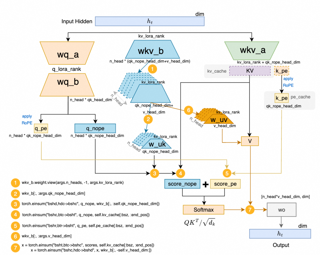
从图中可知,单个 Token 的 KVCache 用量可从 forward 中 kv = self.wkv_a(x) 推出:维度为 kv_lora_rank(512)+ qk_rope_head_dim(64)=576。
使用 ptflops 做复杂度统计(但存在漏算):
args = ModelArgs()
m = MLA(args)
num_tokens = 1

mla_flops, mla_params = get_model_complexity_info(m, (num_tokens,args.dim),as_strings=True,print_per_layer_stat=True)

##输出结果如下
MLA(
187.17 M, 99.999% Params, 170.36 MMac, 100.000% MACs,
  (wq_a): Linear(11.01 M, 5.883% Params, 11.01 MMac, 6.464% MACs, in_features=7168, out_features=1536, bias=True)
  (q_norm): RMSNorm(0, 0.000% Params, 0.0 Mac, 0.000% MACs, (1536,), eps=None, elementwise_affine=True)
  (wq_b): Linear(37.77 M, 20.181% Params, 37.77 MMac, 22.172% MACs, in_features=1536, out_features=24576, bias=True)
  (wkv_a): Linear(4.13 M, 2.206% Params, 4.13 MMac, 2.424% MACs, in_features=7168, out_features=576, bias=True)
  (kv_norm): RMSNorm(0, 0.000% Params, 0.0 Mac, 0.000% MACs, (512,), eps=None, elementwise_affine=True)
  (wkv_b): Linear(16.81 M, 8.981% Params, 0.0 Mac, 0.000% MACs, in_features=512, out_features=32768, bias=True)
  (wo): Linear(117.45 M, 62.748% Params, 117.45 MMac, 68.940% MACs, in_features=16384, out_features=7168, bias=True)
)
单个 MLA block 参数量 187.17M 没问题;但单 token 的 170.36M Mac 实际有误:wkv_b 在 split 为 w_uk 和 w_uv 时算力消耗没被统计。为此定义手工计算函数:
def mla_flops(q_len, kv_len, args:ModelArgs, kv_cache_rate=0):
#calculate MACs and estimate Flops approx. 2xMAC.
    q_down_proj = q_len * args.dim * args.q_lora_rank #wq_a
    q_up_proj = q_len * args.q_lora_rank * args.n_heads * (args.qk_nope_head_dim + args.qk_rope_head_dim) #wq_b
    kv_down_proj = kv_len * args.dim * (args.kv_lora_rank + args.qk_rope_head_dim) #wkv_a
    k_up_proj = kv_len * args.kv_lora_rank * args.n_heads * args.qk_nope_head_dim #w_uk
    v_up_proj = kv_len * args.kv_lora_rank * args.n_heads * args.v_head_dim #w_uv

    kv_down_proj = kv_down_proj * (1 - kv_cache_rate)
    gemm_sum = q_down_proj + q_up_proj + kv_down_proj + k_up_proj + v_up_proj

#把它看成一个标准的args.n_heads的MHA
    mha = args.n_heads * ( q_len * args.qk_rope_head_dim * kv_len #QK_score_rope
                          + q_len * args.qk_nope_head_dim * kv_len #QK_score_nope
                          + q_len * kv_len * args.v_head_dim) #ScoreV
    wo = q_len * args.n_heads * args.v_head_dim * args.dim #wo
    attn_sum = mha + wo

#return flops by 2* Sum(MACs)
    GEMM_FP8_FLOPS = gemm_sum * 2/1e9
    ATTN_FP16_FLOPS =  attn_sum * 2/1e9

return GEMM_FP8_FLOPS+ATTN_FP16_FLOPS, GEMM_FP8_FLOPS,ATTN_FP16_FLOPS
单 token 实际复杂度:
mla_flops(1,1,args,0)

(0.37429248000000004, 0.139329536, 0.234962944)
1.1.2 矩阵吸收模式
DeepSeek-V2 论文提到:
Fortunately, due to the associative law of matrix multiplication, we can absorb 𝑊_𝑈𝐾 into 𝑊𝑈𝑄, and 𝑊_𝑈𝑉 into 𝑊𝑂
其中 WU_Q 对应上文 wq_b。在流程图第 (3) 步前可将 w_uk 与 wq_b 先相乘;第 (7) 步可将 w_uv 与 wo 相乘:
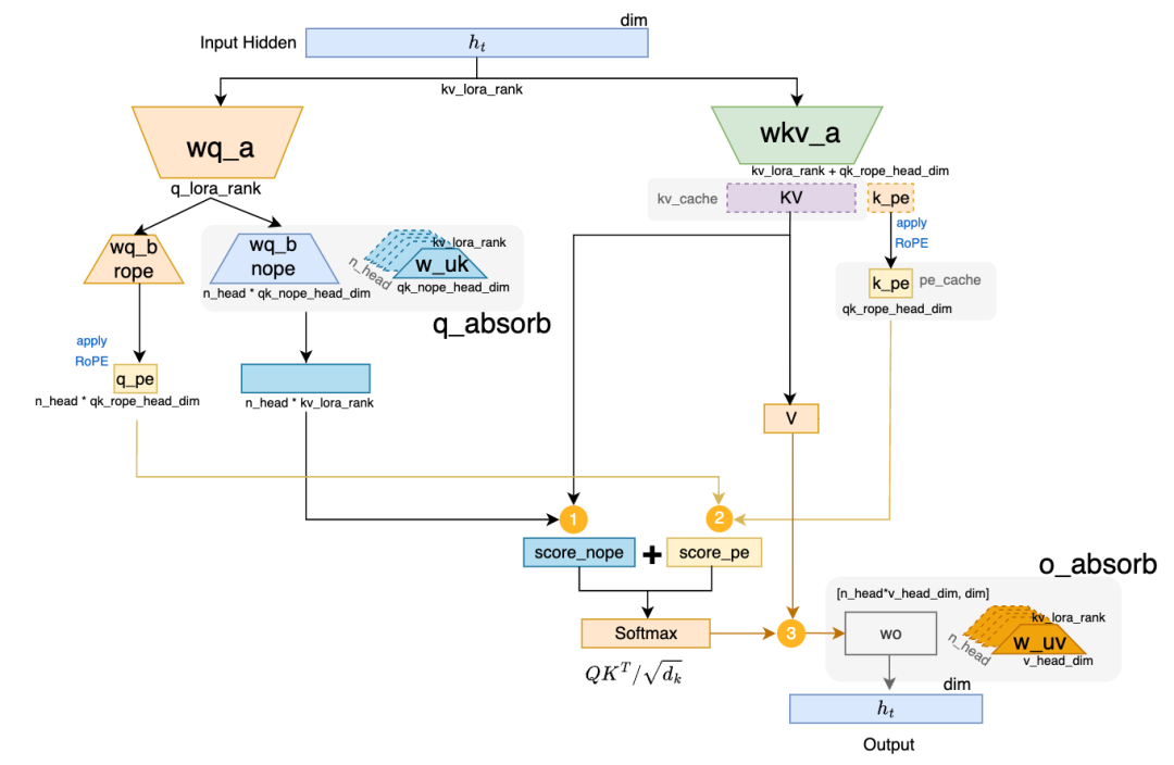
wq_b_nope 为 [q_lora_rank(1536), n_head(128) x qk_nope_head_dim(128)]w_uk 为 [kv_lora_rank(512), n_head(128) x qk_nope_head_dim(128)]
吸收后 q_absorb 为 [q_lora_rank(1536), n_head(128) x kv_lora_rank(512)]。
同理吸收 wo 和 w_uv:
wo 为 [n_head(128) x v_head_dim(128), dim(7168)]w_uv 为 [kv_lora_rank(512), n_head(128) x v_head_dim(128)]
吸收后 o_absorb 为 [dim(7168), n_head(128) x kv_lora_rank(512)]。
对应算力消耗函数:
def mla_matabsob_flops(q_len, kv_len, args:ModelArgs, kv_cache_rate=0):
#calculate MACs and estimate Flops approx. 2xMAC.
    q_down_proj = q_len * args.dim * args.q_lora_rank #wq_a
    q_rope_up_proj = q_len * args.q_lora_rank * args.n_heads * args.qk_rope_head_dim #wq_b_rope
    q_absorb = q_len * args.n_heads * args.q_lora_rank * args.kv_lora_rank

    kv_down_proj = kv_len * args.dim * (args.kv_lora_rank + args.qk_rope_head_dim) #wkv_a
    kv_down_proj = kv_down_proj * (1 - kv_cache_rate) #KV-Cache命中率修正
    gemm_sum = q_down_proj + q_rope_up_proj + q_absorb + kv_down_proj

#把它看成一个标准的args.n_heads的MQA
    mqa = args.n_heads * ( q_len * args.qk_rope_head_dim * kv_len #Score_rope
                          + q_len * args.kv_lora_rank * kv_len #Score_nope
                          + q_len * kv_len * args.kv_lora_rank) #Score V
    o_absorb = q_len * args.n_heads * args.kv_lora_rank * args.dim
    attn_sum = mqa + o_absorb

#return flops by 2* Sum(MACs)
    gemm_sum =  gemm_sum * 2/1e9
    attn_sum = attn_sum * 2/1e9

return gemm_sum + attn_sum, gemm_sum,attn_sum
单 token 复杂度:
mla_matabsob_flops(1,1,args,0)

(1.196572672, 0.256770048, 0.939802624)
相对于非吸收版本:
mla_matabsob_flops(1,1,args,0)[0] / mla_flops(1,1,args,0)[0],运算复杂度反而增加 3.197 倍。
吸收后参数量估计:
def mla_matabsob_mem(args:ModelArgs):
    q_down_proj = args.dim * args.q_lora_rank #wq_a
    q_rope_up_proj =  args.q_lora_rank * args.n_heads * args.qk_rope_head_dim #wq_b_rope
    q_absorb = args.n_heads * args.q_lora_rank * args.kv_lora_rank
    kv_down_proj =  args.dim * (args.kv_lora_rank + args.qk_rope_head_dim) #wkv_a
    o_absorb = args.n_heads * args.kv_lora_rank * args.dim
return q_down_proj + q_rope_up_proj + q_absorb + kv_down_proj + o_absorb

mla_matabsob_mem(args)/1e6
598.147072
参数量也增加到 598.14M(同样约 3.197 倍)。
但 MLA_Absorb 在 Decoding 阶段会有额外收益。根据官方资料《DeepSeek-V3 / R1 推理系统概览》[1],平均每输出一个 token 的 KVCache 长度约为 4989;据此计算两者差异显著:
#Prefill
mla_matabsob_flops(4989,4989,args,0)[0] / mla_flops(4989,4989,args,0)[0]

3.3028

#Decoding时qlen=1,KVcache不需要计算kv_cache_rate=1
mla_matabsob_flops(1,4989,args,1)[0] / mla_flops(1,4989,args,1)[0]

0.015
结论:Prefill 阶段采用非吸收版本,Decoding 阶段采用矩阵吸收版本。
1.2 DenseMLP 计算复杂度
模型前三层采用 Dense MLP:
class DenseMLP(nn.Module):
def __init__(self, dim: int, inter_dim: int):
        super().__init__()
        self.w1 = nn.Linear(dim, inter_dim, dtype=torch.bfloat16)
        self.w2 = nn.Linear(inter_dim, dim, dtype=torch.bfloat16)
        self.w3 = nn.Linear(dim, inter_dim, dtype=torch.bfloat16)

def forward(self, x: torch.Tensor) -> torch.Tensor:
return self.w2(F.silu(self.w1(x)) * self.w3(x))

args = ModelArgs()
#dim=7168,inter_dim=18432
d = DenseMLP(args.dim, args.inter_dim)
num_tokens = 1

mlp_flops, mlp_params = get_model_complexity_info(d, (1,num_tokens,args.dim),as_strings=True,print_per_layer_stat=True)
##输出结果如下:
DenseMLP(
396.41 M, 100.000% Params, 396.41 MMac, 99.995% MACs,
  (w1): Linear(132.14 M, 33.334% Params, 132.14 MMac, 33.333% MACs, in_features=7168, out_features=18432, bias=True)
  (w2): Linear(132.13 M, 33.331% Params, 132.13 MMac, 33.330% MACs, in_features=18432, out_features=7168, bias=True)
  (w3): Linear(132.14 M, 33.334% Params, 132.14 MMac, 33.333% MACs, in_features=7168, out_features=18432, bias=True)
)
单个 MLP block 参数量 396.41M,单 token 计算复杂度约 396.41M Mac(约 792.82 MFLOPS)。定义计算复杂度函数:
def densmlp_flops(args:ModelArgs, seq_len):
return 3 * seq_len * args.dim * args.inter_dim *2 /1e9
1.3 MoE Expert 计算复杂度
后 58 层采用 MoE,其 Expert 计算复杂度:
class Expert(nn.Module):
def __init__(self, dim: int, inter_dim: int):
        super().__init__()
        self.w1 = nn.Linear(dim, inter_dim, dtype=torch.bfloat16)
        self.w2 = nn.Linear(inter_dim, dim, dtype=torch.bfloat16)
        self.w3 = nn.Linear(dim, inter_dim, dtype=torch.bfloat16)

def forward(self, x: torch.Tensor) -> torch.Tensor:
return self.w2(F.silu(self.w1(x)) * self.w3(x))
args = ModelArgs()
num_tokens = 1

#dim=7168,moe_inter_dim=2048
e = Expert(args.dim, args.moe_inter_dim)

moe_flops, moe_params = get_model_complexity_info(e, (1,num_tokens,args.dim),as_strings=True,print_per_layer_stat=True)
##输出结果如下:
Expert(
44.05 M, 100.000% Params, 44.05 MMac, 99.995% MACs,
  (w1): Linear(14.68 M, 33.329% Params, 14.68 MMac, 33.328% MACs, in_features=7168, out_features=2048, bias=True)
  (w2): Linear(14.69 M, 33.341% Params, 14.69 MMac, 33.340% MACs, in_features=2048, out_features=7168, bias=True)
  (w3): Linear(14.68 M, 33.329% Params, 14.68 MMac, 33.328% MACs, in_features=7168, out_features=2048, bias=True)
)
单个 Expert 参数量 44.05M,单 token 计算复杂度约 44.05M Mac(约 88.1 MFLOPS)。定义计算复杂度函数:
def moe_expert_flops(args:ModelArgs, seq_len):
return 3 * seq_len * args.dim * args.moe_inter_dim *2/1e9
1.4 数据汇总
模型整体参数分布如下(另有 MoE Gating 参数 dim x n_routed_expert + n_routed_expert(bias)=1.83M,以及 Embedding/Output 参数 vocab_size x dim=926.67M)。
| Block |
单层参数量 |
层数 |
累计参数 |
| MLA |
187.17M |
61 |
11.41B |
| DenseMLP |
396.41M |
3 |
1.19B |
| Expert |
44.05Mx(256_routed+1_shared) |
58 |
656.6B |
| Gate |
1.83M |
58 |
106.14M |
| Embedding |
926.67M |
1 |
926.67M |
| Output |
926.67M |
1 |
926.67M |
| SUM |
- |
- |
671.16B |
不同 block 的算力消耗统计:
| Block |
参数量 |
运算复杂度(FLops) |
KVCache用量 |
| MLA |
187.17M |
374.29M |
576B(FP8) |
| MLA_absorb |
598.14M |
1196.57M |
576(FP8) |
| DenseMLP |
396.41M |
792.82M |
- |
| Expert |
44.05M |
488.1M |
- |
实际评估会结合 Prefill/Decode 阶段,以及 KVCache 命中率。
KVCache 用量:单个 Token 的 KVCache 累积 61 层;按 FP16 保存为 2 x 576 x 61 = 68.62KB,按 FP8 保存为 34.31KB。
H20/H800 指标如下:
| GPU类型 |
SM |
FP16算力 |
FP8算力 |
显存大小 |
显存带宽 |
NVLINK带宽 |
PCIe带宽 |
| H800 |
132 |
989.5 |
1979 |
80GB |
3350 |
200 |
50 |
| H20 |
78 |
148 |
296 |
96GB |
3350 |
450 |
50 |
为了便于后续计算,定义 GPU 性能函数,整体性能按峰值 85% 估计。H800 需要 24 个通信 SM;考虑 H20 浮点算力较弱,估计 H20 需要 10 个通信 SM:
class GPU_perf():
def __init__(self,sm,comm_sm, fp16_flops,fp8_flops,mem,mem_bw, nvlink_bw,pcie_bw, discount_rate):
        self.sm = sm
        self.comm_sm = comm_sm #用于通信的SM数量
        self.fp16_flops = fp16_flops
        self.fp8_flops = fp8_flops
        self.mem = mem
        self.mem_bw = mem_bw
        self.nvlink_bw = nvlink_bw
        self.pcie_bw = pcie_bw
        self.discount_rate = discount_rate #整体性能按峰值性能折扣
#TODO: 可以分离网络性能折扣和算力性能折扣

def get_fp16_flops(self):
return self.fp16_flops * self.discount_rate  * ( self.sm  - self.comm_sm) / self.sm

def get_fp8_flops(self):
return self.fp8_flops *  self.discount_rate * ( self.sm  - self.comm_sm) / self.sm

def get_mem_bw(self):
return self.mem_bw *  self.discount_rate

def get_nvlink_bw(self):
return self.nvlink_bw *  self.discount_rate

def get_pcie_bw(self):
return self.pcie_bw *  self.discount_rate

h800 = GPU_perf( sm = 132 ,comm_sm = 24,
                 fp16_flops = 791.6, fp8_flops = 1583.2,
                 mem = 80,mem_bw = 3350,
                 nvlink_bw = 200,pcie_bw = 50,
                 discount_rate = 0.85)

h20 = GPU_perf( sm = 78 ,comm_sm = 10,
                 fp16_flops = 118.4, fp8_flops = 236.8,
                 mem = 96,mem_bw = 3350,
                 nvlink_bw = 400,pcie_bw = 50,
                 discount_rate = 0.85)

gpu = dict({'H800': h800, 'H20': h20})
2. Prefill 阶段
根据 DeepSeek 官方报告:Prefill 采用 路由专家 EP32、MLA 和共享专家 DP32。最小部署单元为 4 节点共 32 GPU;每张卡 9 个路由专家 + 1 个共享专家。论文中 attention 并行策略:
The minimum deployment unit of prefilling stage consists of 4 nodes with 32 GPUs. The attention part employs 4-way Tensor Parallelism (TP4) with Sequence Parallelism (SP), combined with 8-way Data Parallelism (DP8). For the MoE part, we use 32-way Expert Parallelism (EP32)
从 Attention 视角:推理请求在 API Server 通过负载均衡以 DP=8 分配到不同 Prefill 节点的 DP 组内;每个 DP 组内 4 张 H800 组成 TP+SP 组进行 MLA。
从 MoE 视角:32 GPU 组成 EP32 组;每层 256 个 Expert 平均每卡 8 个 routed expert;每卡还有 1 个 shared expert,并按论文还承载 1 个 redundant expert,总计约 10 个 Expert。
这类并行拆分/通信-计算权衡,本质是典型的 分布式系统 工程问题:算力、内存带宽、网络带宽要一起算。
2.1 MLA 计算耗时
参考《DeepSeek V3/R1 推理效率分析(2): DeepSeek 满血版逆向工程分析》[2] 中对 Prefill/Decoding 长度估计:
假设 P 代表平均输入长度,D 代表平均输出长度,则平均每输出 token 的 KVcache 长度约等于 P + D/2 = 4989;再加上 P/D = 608B/168B;P≈4383,D≈1210。
以平均 Prefill seq_len=4383 计算,KVCache 命中率取官方 56.3%,GPU 性能取峰值 85%。
计算函数如下(考虑 TP 并行;假设 seq_len 中有 56.3% 可以从 KVCache 提取,则 Prefill 仅需计算 (1-kv_cache_rate) 的 token):
def prefill_mla_elapse_time(args:ModelArgs,gpu:GPU_perf, discount, comm_sm, seq_len, kv_cache_rate):
    _ , gemm_fp8_flops, attn_fp16_flops = mla_flops(q_len,kv_len,args, 1)
    gemm_fp8_time = gemm_fp8_flops / gpu.get_fp8_flops(discount, comm_sm)
    print("GEMM_FP8 Elapsed time(ms): %.3f" % gemm_fp8_time)
    attn_fp16_time = attn_fp16_flops / gpu.get_fp16_flops(discount, comm_sm)
    print("ATTN_FP16 Elapsed time(ms): %.3f" % attn_fp16_time)
    total_time = gemm_fp8_time + attn_fp16_time
    print("Total Elapsed time(ms):%.3f" % total_time)

    all_reduce_comm_size = seq_len * args.dim * 2 /1024/1024#fp16 take 2Bytes
    ar_elapsed_time = all_reduce_comm_size / gpu.get_nvlink_bw(discount)
    print("AR Elapsed time(ms):%.3f" % ar_elapsed_time)

    tp4_time = total_time/4 + ar_elapsed_time
    print("TP4 Elapsed time(ms):%.3f" % tp4_time)

    tp8_time = total_time/8 + ar_elapsed_time
    print("TP8 Elapsed time(ms):%.3f" % tp8_time)
return total_time, tp4_time,tp8_time

def prefill_mla(args:ModelArgs, gpu_dict, seq_len, kv_cache_rate):
    df = pd.DataFrame(columns=['GPU','TP1','TP4','TP8'])
for key in gpu_dict.keys():
        print('------------ %s --------------' % key)
        tp1,tp4,tp8 = prefill_mla_elapse_time(args,gpu_dict[key], seq_len, kv_cache_rate)
        df.loc[len(df)]=[key,tp1,tp4,tp8]
    print(df.set_index('GPU').to_markdown(floatfmt=".3f"))
H800 24 个通信 SM;H20 10 个通信 SM,同时计算 TP=4 和 TP=8。TP 并行 AllReduce 通信量为 seq_len x dim x 2Bytes(BF16)。
seq_len = 4383
kv_cache_rate = 0.563

prefill_mla(args,gpu,seq_len,kv_cache_rate)
------------ H800 --------------
GEMM_FP8 Elapsed time(ms): 0.536
ATTN_FP16 Elapsed time(ms): 4.729
Total Elapsed time(ms):5.265
AR Elapsed time(ms):0.352
TP4 Elapsed time(ms):1.669
TP8 Elapsed time(ms):1.011
------------ H20 --------------
GEMM_FP8 Elapsed time(ms): 3.364
ATTN_FP16 Elapsed time(ms): 29.671
Total Elapsed time(ms):33.035
AR Elapsed time(ms):0.176
TP4 Elapsed time(ms):8.435
TP8 Elapsed time(ms):4.306
MLA 的 GPU 计算时间(ms)汇总:
| GPU |
TP1 |
TP4 |
TP8 |
| H800 |
5.265 |
1.669 |
1.011 |
| H20 |
33.035 |
8.435 |
4.306 |
2.2 DenseMLP 计算耗时
DenseMLP 运算量函数:
def densmlp_flops(args:ModelArgs, seq_len):
return 3 * seq_len * args.dim * args.inter_dim *2 /1e9

def dense_mlp_elapse_time(args:ModelArgs,gpu:GPU_perf, seq_len):
    gemm_fp8_flops = densmlp_flops(args, seq_len)
    gemm_fp8_time = gemm_fp8_flops / gpu.get_fp8_flops()
    print("Elapsed time(ms): %.3f" % gemm_fp8_time)
return gemm_fp8_time

def prefill_dense_mlp(args:ModelArgs, gpu_dict, seq_len):
    df = pd.DataFrame(columns=['GPU','DenseMLP耗时'])
for key in gpu_dict.keys():
        print('------------ %s --------------' % key)
        t = dense_mlp_elapse_time(args,gpu_dict[key], seq_len)
        df.loc[len(df)]=[key,t]
    print(df.set_index('GPU').to_markdown(floatfmt=".3f"))
实际运算长度:
q_len = seq_len *( 1- kv_cache_rate)
------------ H800 --------------
Elapsed time(ms): 3.156
------------ H20 --------------
Elapsed time(ms): 19.801
DenseMLP 累计耗时(ms):
| GPU |
DenseMLP耗时 |
| H800 |
3.156 |
| H20 |
19.801 |
2.3 MoE 计算耗时
TP=4 时,DP=8,相当于 MLA 同时产生 8 组 seq_len token。每卡 shared expert 处理 token 数约为 seq_len * dp_group / num_gpu。
对 routed expert:topk=8 时,总 routed token 计算量为 seq_len * dp_group * topk,平均摊到 32 卡,每卡 routed token 为 seq_len * dp_group * topk / num_gpu。
def moe_expert_flops(args:ModelArgs, seq_len):
return 3 * seq_len * args.dim * args.moe_inter_dim *2/1e9

def moe_expert_elapse_time(args:ModelArgs,gpu:GPU_perf, seq_len, tp, dp):
    num_device = tp * dp
    num_shared_token = dp * seq_len / num_device
    shared_flops = moe_expert_flops(args, num_shared_token)
    shared_time = shared_flops / gpu.get_fp8_flops()
    print("Shared Expert Elapsed time(ms): %.3f" % shared_time)

    num_routed_token = seq_len * dp * args.n_activated_experts / num_device
    routed_flops = moe_expert_flops(args, num_routed_token)
    routed_time = routed_flops / gpu.get_fp8_flops()
    print("Routed Expert Elapsed time(ms): %.3f" % routed_time)

return shared_time, routed_time

def prefill_moe(args:ModelArgs, gpu_dict, seq_len, tp, dp ):
    df = pd.DataFrame(columns=['GPU','Shared Expert','Routed Expert'])
for key in gpu_dict.keys():
        print('------------ %s --------------' % key)
        s, r = moe_expert_elapse_time(args,gpu_dict[key], seq_len,tp,dp)
        df.loc[len(df)]=[key,s,r]
    print(df.set_index('GPU').to_markdown(floatfmt=".3f"))
TP=4,DP=8:
prefill_moe(args,gpu, seq_len, tp=4,dp=8)
------------ H800 --------------
Shared Expert Elapsed time(ms): 0.088
Routed Expert Elapsed time(ms): 0.701
------------ H20 --------------
Shared Expert Elapsed time(ms): 0.550
Routed Expert Elapsed time(ms): 4.400
| GPU |
Shared Expert |
Routed Expert |
| H800 |
0.088 |
0.701 |
| H20 |
0.550 |
4.400 |
TP=8,DP=4:
prefill_moe(args,gpu, seq_len, tp=8,dp=4)
------------ H800 --------------
Shared Expert Elapsed time(ms): 0.044
Routed Expert Elapsed time(ms): 0.351
------------ H20 --------------
Shared Expert Elapsed time(ms): 0.275
Routed Expert Elapsed time(ms): 2.200
| GPU |
Shared Expert |
Routed Expert |
| H800 |
0.044 |
0.351 |
| H20 |
0.275 |
2.200 |
2.4 AlltoAll 通信耗时
DeepSeek-V3 设计了 MoE Group 用于平衡 NVLINK 与 IB 带宽:一个 token 通过 gating 后最多只会分发到 4 个节点。假设 EP 负载完全均衡,跨机 RDMA 通信约为 3 * token数。
Dispatch 通信量估计:
- TP=4:每节点 2 个 DP 组,需要发送
2 * 3 * seq_len * dim
- TP=8:每节点 1 个 DP 组,需要发送
3 * seq_len * dim
Combine 阶段 FP16,通信量翻倍。H800/H20 ScaleOut 带宽相同,按 DeepEP 约 45GB/s,考虑利用率取 80%(约 40GB/s),总带宽 40GB/s * 8 = 320GB/s。
def prefill_alltoall_time(args:ModelArgs, gpu, seq_len, dispatch_node, tp):
##通信量估计
    gpu_per_node = 8
    dp = gpu_per_node/tp
    dispatch_size = (dispatch_node - 1) * dp * seq_len * args.dim /1024/1024
    combine_size = 2 * dispatch_size  #fp16
    comm_bw = gpu.get_pcie_bw() * gpu_per_node
    dispatch_time = dispatch_size / comm_bw
    combine_time = combine_size / comm_bw
return dispatch_time, combine_time

def prefill_alltoall(args:ModelArgs, gpu_dict, seq_len, dispatch_node, tp):
    df = pd.DataFrame(columns=['GPU','Dispatch','Combine'])
for key in gpu_dict.keys():
        print('------------ %s --------------' % key)
        dispatch_time, combine_time = prefill_alltoall_time(args, gpu_dict[key],seq_len, dispatch_node, tp)
        print("Dispatch Elapsed time(ms): %.3f" % dispatch_time)
        print("Combine Elapsed time(ms): %.3f" % combine_time)
        df.loc[len(df)]=[key,dispatch_time,combine_time]
    print(df.set_index('GPU').to_markdown(floatfmt=".3f"))
TP=4(每节点 2 个 DP 组):
prefill_alltoall(args,gpu,seq_len,dispatch_node=4,tp=4)
------------ H800 --------------
Dispatch Elapsed time(ms): 0.529
Combine Elapsed time(ms): 1.057
------------ H20 --------------
Dispatch Elapsed time(ms): 0.529
Combine Elapsed time(ms): 1.057
| GPU |
Dispatch |
Combine |
| H800 |
0.529 |
1.057 |
| H20 |
0.529 |
1.057 |
TP=8(每节点 1 个 DP 组):
prefill_alltoall(args,gpu,seq_len,dispatch_node=4,tp=8)
------------ H800 --------------
Dispatch Elapsed time(ms): 0.264
Combine Elapsed time(ms): 0.529
------------ H20 --------------
Dispatch Elapsed time(ms): 0.264
Combine Elapsed time(ms): 0.529
| GPU |
Dispatch |
Combine |
| H800 |
0.264 |
0.529 |
| H20 |
0.264 |
0.529 |
2.5 总耗时
累计耗时(非 Overlap):
3x(MLA_tp1 + DenseMLP) + 58x(MLA_tpN + Shared Expert + Routed Expert +Dispatch + Combine)
累计耗时(完全 Overlap):
3x(MLA_tp1 + DenseMLP) + 58x(MLA_tpN + Shared Expert + Routed Expert)
计算函数:
def prefill_time(args:ModelArgs, gpu, seq_len, kv_cache_rate, tp , dp):
    dispatch_node = 4
    gpu_per_node = 8
    num_device  =  tp * dp
    dense_mla,tp4_mla,tp8_mla = prefill_mla_elapse_time(args, gpu,  seq_len, kv_cache_rate)
    tp_mla = tp4_mla if tp == 4 else tp8_mla
    dense_mlp = dense_mlp_elapse_time(args, gpu, seq_len)
    shared, routed = moe_expert_elapse_time(args, gpu, seq_len, tp, dp)
    dispatch, combine = prefill_alltoall_time(args, gpu, seq_len, dispatch_node, tp)
return dense_mla, dense_mlp, tp_mla, shared, routed, dispatch, combine

def prefill_time_sum(args:ModelArgs, gpu_dict, seq_len, kv_cache_rate, tp , dp):
    df = pd.DataFrame(columns=['MLA','DenseMLP','TP_MLA','Shared Expert','Routed Expert','Dispatch','Combine','GPU'])
    df2 = pd.DataFrame(columns=['Sum(Overlap)','Sum','GPU'])
    n_sparse_layers = args.n_layers - args.n_dense_layers
    df.loc[len(df)]= [ args.n_dense_layers, args.n_dense_layers,  #MLA+ DenseMLP
                       n_sparse_layers, n_sparse_layers, n_sparse_layers, #SparseLayer MLA + MoE
                       n_sparse_layers, n_sparse_layers, 'Layers'] #Dispatch & Combine Layers
for key in gpu_dict.keys():
        t  = list(prefill_time(args, gpu_dict[key], seq_len, kv_cache_rate , tp , dp))
        t.append(key)
        df.loc[len(df)]= t
        sum_overlap = args.n_dense_layers * (t[0] + t[1]) + n_sparse_layers * ( t[2] + t[3] + t[4])
        sum_non_overlap = sum_overlap + n_sparse_layers * ( t[5] + t[6]) #alltoall
        df2.loc[len(df2)]= [ sum_overlap, sum_non_overlap, key]
    df = df.set_index('GPU').T
    df['Layers'] = df['Layers'].astype(int).astype(str)
    print(df.to_markdown(floatfmt=".3f"))
    print('-----------SUM-------------')
    df2 = df2.set_index('GPU').T
    print(df2.to_markdown(floatfmt=".3f"))

return df,df2
TP=4,DP=8(ms):
tp4_detail,tp4_sum = prefill_time_sum(args, gpu, seq_len, kv_cache_rate,tp=4 , dp=8)
|
Layers |
H800 |
H20 |
| MLA |
3 |
5.265 |
33.035 |
| DenseMLP |
3 |
3.156 |
19.801 |
| TP_MLA |
58 |
1.669 |
8.435 |
| Shared Expert |
58 |
0.088 |
0.550 |
| Routed Expert |
58 |
0.701 |
4.400 |
| Dispatch |
58 |
0.529 |
0.529 |
| Combine |
58 |
1.057 |
1.057 |
累计时间(ms):
|
H800 |
H20 |
| Sum(Overlap) |
167.802 |
934.839 |
| Sum |
259.803 |
1026.840 |
TP=8,DP=4(ms):
tp8_detail,tp8_sum = prefill_time_sum(args, gpu, seq_len, kv_cache_rate,tp=8 , dp=4)
|
Layers |
H800 |
H20 |
| MLA |
3 |
5.265 |
33.035 |
| DenseMLP |
3 |
3.156 |
19.801 |
| TP_MLA |
58 |
1.011 |
4.306 |
| Shared Expert |
58 |
0.044 |
0.275 |
| Routed Expert |
58 |
0.351 |
2.200 |
| Dispatch |
58 |
0.264 |
0.264 |
| Combine |
58 |
0.529 |
0.529 |
累计时间(ms):
|
H800 |
H20 |
| Sum(Overlap) |
106.754 |
551.784 |
| Sum |
152.754 |
597.784 |
由于累计为 DP 组 seq_len 的推理,平均 1s 单机可处理 token 数为:
DP * seq_len * (1000ms / 计算时间) / 节点数
官方 TP=4 部署方式:
dp = 8
num_node = 4
print(tp4_sum.apply(lambda x: dp * seq_len * (1000/ x)/num_node).to_markdown(floatfmt=".1f"))
|
H800 |
H20 |
| Sum(Overlap) |
52240.1 |
9377.0 |
| Sum |
33741.0 |
8536.9 |
TP=8 部署方式吞吐:
|
H800 |
H20 |
| Sum(Overlap) |
41057.0 |
7943.3 |
| Sum |
28693.1 |
7332.1 |
可见官方选择 TP=4 的配置是吞吐更优的选择。官方数据为单机 73.7K tokens/s(含缓存命中),折算非命中需要计算的平均 token/s 为 32207;考虑峰谷效应,该值符合预期。
另一方面,H20 对 TTFT(首 token 延迟)影响较大:TP=4 已超过 1s,可采用 TP=8 降低首 token 延迟。
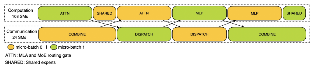
2.6 Overlap 分析
官方部署方案可按两个 micro-batch 做 overlap:
对 prefill.json trace 标注如下(实际 trace 仍有部分未 overlap):

TP=4 时 Prefill 计算耗时关键项(ms)如下,可看到通信可被计算 overlap:
|
Layers |
H800 |
H20 |
| TP_MLA |
58 |
1.669 |
8.435 |
| Shared Expert |
58 |
0.088 |
0.550 |
| Combine |
58 |
1.057 |
1.057 |
| - |
- |
- |
- |
| Routed Expert |
58 |
0.701 |
4.400 |
| Dispatch |
58 |
0.529 |
0.529 |
特别地,针对 H20 还可以降低 RDMA ScaleOut 带宽,做初步估计:
h20_32 = GPU_perf( sm = 78 ,comm_sm = 10,
                 fp16_flops = 118.4, fp8_flops = 236.8,
                 mem = 96,mem_bw = 3350,
                 nvlink_bw = 400,pcie_bw = 50,
                 discount_rate = 0.85)

h20_16 = GPU_perf( sm = 78 ,comm_sm = 10,
                 fp16_flops = 118.4, fp8_flops = 236.8,
                 mem = 96,mem_bw = 3350,
                 nvlink_bw = 400,pcie_bw = 25,
                 discount_rate = 0.85)

h20_8 = GPU_perf( sm = 78 ,comm_sm = 10,
                 fp16_flops = 118.4, fp8_flops = 236.8,
                 mem = 96,mem_bw = 3350,
                 nvlink_bw = 400,pcie_bw = 12.5,
                 discount_rate = 0.85)

gpu_h20 = dict({ 'H20-3.2T': h20_32, 'H20-1.6T': h20_16 , 'H20-800G': h20_8})
tp4_detail,tp4_sum = prefill_time_sum(args, gpu_h20, seq_len, kv_cache_rate,tp=4 , dp=8)
|
Layers |
H20-3.2T |
H20-1.6T |
H20-800G |
| TP_MLA |
58 |
8.435 |
8.435 |
8.435 |
| Shared Expert |
58 |
0.550 |
0.550 |
0.550 |
| Dispatch |
58 |
0.529 |
1.057 |
2.115 |
| - |
- |
- |
- |
- |
| Routed Expert |
58 |
4.400 |
4.400 |
4.400 |
| Combine |
58 |
1.057 |
2.115 |
4.230 |
|
H20-3.2T |
H20-1.6T |
H20-800G |
| Sum(Overlap) |
934.839 |
934.839 |
934.839 |
| Sum |
1026.840 |
1118.841 |
1302.842 |
- 注:若大量 Prefill 长度在 1000~2000 左右,仍需要 1.6Tbps~3.2Tbps RDMA。
2.7 KVCache 计算
将 token/s 折算为 KVCache 传输总量:
dp = 8
num_node = 4

tp4_detail,tp4_sum = prefill_time_sum(args, gpu, seq_len, kv_cache_rate,tp=4 , dp=8)
kvcache_fp8 = tp4_sum.apply(lambda x: dp * seq_len * (1000/ x)/num_node * (args.kv_lora_rank + args.qk_rope_head_dim)/1024/1024)
kvcache_fp16 = kvcache_fp8 *2
kvcache=kvcache_fp8.join(kvcache_fp16, lsuffix='(FP8)',rsuffix='(FP16)')
print(kvcache.to_markdown(floatfmt=".1f"))
| GB/s |
H800(FP8) |
H20(FP8) |
H800(FP16) |
H20(FP16) |
| Sum(Overlap) |
28.7 |
5.2 |
57.4 |
10.3 |
| Sum |
18.5 |
4.7 |
37.1 |
9.4 |
- 注:未考虑 KVCache 命中率;考虑后带宽应体现读写两个方向。
对 H800 而言,如果 KVCache 采用 FP16 存储,已超过连接 CPU 的 400Gbps(50GB/s)网卡带宽,需要采用 GPU 直连 RDMA 的 ScaleOut 网络进行传输;而在合理编排通信算子并保证 EP 并行实现恰当的情况下,对整体影响可以做到接近可忽略。
3. Decoding 阶段
Decoding 集群采用 18 台部署:路由专家 EP144,MLA 与共享专家 DP144;32 个冗余路由专家;每卡 2 个路由专家 + 1 个共享专家。论文做法为 40 台部署 EP320,每卡 1 个专家,TP=4,DP=80。Decode 阶段不需要独立通信 SM,GPU 性能建模如下:
h800 = GPU_perf( sm = 132 ,comm_sm = 0,
                 fp16_flops = 791.6, fp8_flops = 1583.2,
                 mem = 80,mem_bw = 3350,
                 nvlink_bw = 200,pcie_bw = 50,
                 discount_rate = 0.85)

h20 = GPU_perf( sm = 78 ,comm_sm = 0,
                 fp16_flops = 118.4, fp8_flops = 236.8,
                 mem = 96,mem_bw = 3350,
                 nvlink_bw = 400,pcie_bw = 50,
                 discount_rate = 0.85)
h20_3e = GPU_perf( sm = 78 ,comm_sm = 0,
                 fp16_flops = 118.4, fp8_flops = 236.8,
                 mem = 141,mem_bw = 4800,
                 nvlink_bw = 400,pcie_bw = 50,
                 discount_rate = 0.85)

gpu_decode = dict({'H800': h800, 'H20': h20,'H20_3e': h20_3e})
gpu_decode2 = dict({'H800': h800, 'H20': h20})
3.1 EP 策略分析
线上常见 Expert 负载不均衡,需要足够冗余专家用于 EPLB 调度。设冗余专家数不低于 16,常见 EP 策略:
|
冗余专家 |
每卡专家 |
| EP34 |
16 |
8 |
| EP72 |
32 |
4 |
| EP144 |
32 |
2 |
| EP320 |
64 |
1 |
不同并行策略下通信/计算 token 数估计:
class MoE_EP():
def __init__(self,args:ModelArgs,ep_num, redundant_exp):
        self.ep_num = ep_num
        self.redundant_exp = redundant_exp
        self.dispatch_num = args.n_activated_experts
        self.n_routed_experts = args.n_routed_experts
        self.expert_num = (args.n_routed_experts + redundant_exp) / self.ep_num

def expert_per_gpu(self):
return self.expert_num

def total_tokens(self,bs):
return bs * self.ep_num

def comm_tokens(self, bs):
#平均每个token有self.expert_num / self.n_routed_experts概率本地处理
return bs * self.dispatch_num *(1- self.expert_num / self.n_routed_experts)

def compute_tokens(self, bs):
#总token数为bs * dispatch_num * ep_num, 平摊到每张卡/ep_num
return bs * self.dispatch_num

ep_dict = { 'EP34': MoE_EP(args, 34,16),
'EP72' :MoE_EP(args, 72,32),
'EP144' :MoE_EP(args, 144,32),
'EP320' :MoE_EP(args, 320,64)}
3.2 Memory 利用率分析
先从显存容量推导最大 BatchSize。Decoding 阶段采用 matabsorb MLA。除去 MLA 与 Expert 参数后,其它参数为:
671.16B - MLA(187.17M)* 61 - Expert(44.05M)* (256-Routed+1-Shared) * 58 = 3.13B
折算显存约 3.13 * (1000/1024)^3 = 2.91GB。
BatchSize 计算如下(Decoding 长度 1210;按 EP 策略估计专家数):
def _decoding_batchsize(args:ModelArgs, gpu:GPU_perf, seq_len,decode_len,tp, expert_num, absorb=True, kvcache_fp16=False):
    mem_util_rate = 0.9#torch/activation等其它开销的折扣
    mla = 598.14 if absorb else 187.17#MLA的参数(单位M)
    expert_mem = 44.05#expert的参数(单位M)
    others_parameter = 2.91#其它参数2.91GB
    kv_cache = (seq_len+decode_len) * (args.kv_lora_rank + args.qk_rope_head_dim) *args.n_layers *tp
if kvcache_fp16 :
        kv_cache *=2
    mem = gpu.mem * mem_util_rate - others_parameter - mla * args.n_layers/tp/1024
    mem -= expert_mem *(args.n_layers - args.n_dense_layers) * expert_num /1024
return mem * 1024 * 1024 * 1024 / kv_cache

def decode_batchsize(args:ModelArgs, gpu_dict, seq_len,decode_len, tp):
    df = pd.DataFrame(columns=['GPU','EP320','EP144','EP72','EP34'])
for fp16_kvcache in range(0,2):
for key in gpu_dict.keys():
for absorb in range(0,2):
                item = key
if bool(fp16_kvcache):
                    item +='_FP16'
else:
                    item +='_FP8'
if bool(absorb):
                    item +='_Absorb'
                value = [item]
for exp_num in [2,3,5,9]:
                    bs = _decoding_batchsize(args, gpu_dict[key], seq_len,decode_len, tp,exp_num, bool(absorb),bool(fp16_kvcache))
                    value.append(bs)
                df.loc[len(df)]= value
    print(df.set_index('GPU').to_markdown(floatfmt=".0f"))
return df

decode_len = 1210
df = decode_batchsize(args,gpu_decode, seq_len,decode_len, tp=1)
(以下为原统计表,略)
结论要点:
- 显存越大越容易放下足够 BatchSize。
- 需要保证每卡路由专家数不超过 8。
- H800 在 MLA 矩阵吸收模式下,需要 KVCache 用 FP8 存储才能满足
batchsize=128 需求。
3.3 MLA 耗时
Decoding 使用矩阵吸收 MLA。由于计算延迟较低,还要计入加载 KVCache 的时间。
bs_list =[32, 64, 128, 256]

def decode_mla_elapse_time(args:ModelArgs, gpu:GPU_perf, seq_len, bs, absorb=True):
    mla_flops_func = mla_matabsob_flops if absorb else mla_flops
#Decoding时计算为qlen=1, kv_cache_rate = 1
    _ , gemm_fp8_flops, attn_fp16_flops = mla_flops_func(1,seq_len,args, 1)

    gemm_fp8_time = gemm_fp8_flops / gpu.get_fp8_flops() * bs
    print("GEMM_FP8 Elapsed time(ms): %.3f" % gemm_fp8_time)
    attn_fp16_time = attn_fp16_flops / gpu.get_fp16_flops() *bs
    print("ATTN_FP16 Elapsed time(ms): %.3f" % attn_fp16_time)
    total_time = gemm_fp8_time + attn_fp16_time
    print("Total Elapsed time(ms):%.3f" % total_time)
    all_reduce_comm_size = seq_len * args.dim * 2 /1024/1024#fp16 take 2Bytes
    ar_elapsed_time = all_reduce_comm_size / gpu.get_nvlink_bw()
    print("AR Elapsed time(ms):%.3f" % ar_elapsed_time)
    tp4_time = total_time/4 + ar_elapsed_time
    print("TP4 Elapsed time(ms):%.3f" % tp4_time)
    tp8_time = total_time/8 + ar_elapsed_time
    print("TP8 Elapsed time(ms):%.3f" % tp8_time)
return total_time, tp4_time, tp8_time

def decode_kvcache_load_time(args:ModelArgs, gpu:GPU_perf, seq_len, bs):
    kv_cache = seq_len * (args.kv_lora_rank + args.qk_rope_head_dim)  * bs
    load_kv_time = kv_cache /1024/1024/1024 / gpu.get_mem_bw() *1000
return load_kv_time

def decode_mla(args:ModelArgs, gpu_dict, seq_len,absorb=True):
    df = pd.DataFrame(columns=['GPU','BatchSize','TP1','TP4','TP8','LoadKV_FP8','LoadKV_FP16'])
for key in gpu_dict.keys():
for bs in bs_list:
             tp1, tp4,tp8 = decode_mla_elapse_time(args,gpu_dict[key], seq_len, bs,absorb)
             kv = decode_kvcache_load_time(args,gpu_dict[key], seq_len, bs)
             df.loc[len(df)]= [key, bs,tp1,tp4,tp8,kv, kv*2]
             df['BatchSize'] = df['BatchSize'].astype(int).astype(str)
    print(df.set_index('GPU').to_markdown(floatfmt=".3f"))
return df
(以下为原统计表,略)
结论要点:
- H800/H20 在 Decoding 阶段都需要使用矩阵吸收 MLA。
- H800:在
batchsize=128 时 TP=4 与 TP1 耗时相近,batchsize=64 时甚至更快;因此 EP144 部署中不必强制 TP。
- H20:MLA 必须使用 TP 并行;但 TP 过大增加 KVCache 开销并限制 batchsize,综合最优为 TP=4。
3.4 DenseMLP 耗时
def decode_dense_mlp(args:ModelArgs, gpu_dict):
    df = pd.DataFrame(columns=['GPU','BatchSize','DenseMLP'])
for key in gpu_dict.keys():
for bs in bs_list:
            t = dense_mlp_elapse_time(args,gpu_dict[key], bs)
            df.loc[len(df)]=[key,bs,t]
    df['BatchSize'] = df['BatchSize'].astype(int).astype(str)
    print(df.set_index('GPU').to_markdown(floatfmt=".3f"))
return df

decode_dense_mlp(args,gpu_decode)
(以下为原统计表,略)
3.5 MoE 耗时计算
简化:任何 token 都要 dispatch 8 份到其它节点;考虑 GroupGEMM 在小 batch 下难以打满,按 DeepGEMM 设折算系数 0.7。
def _moe_expert_time(args:ModelArgs,gpu:GPU_perf,bs):
    group_gemm_discount_rate = 0.7
    shared_flops = moe_expert_flops(args, bs)
    shared_time = shared_flops / gpu.get_fp8_flops() / group_gemm_discount_rate

    num_routed_token = bs * args.n_activated_experts
    routed_flops = moe_expert_flops(args, num_routed_token)
    routed_time = routed_flops / gpu.get_fp8_flops() / group_gemm_discount_rate
return shared_time, routed_time
(以下为原统计表,略)
3.5 AlltoAll 通信耗时
IBGDA 方式直接 RDMA 传输,计算时主要考虑 GPU PCIe 带宽:
def _moe_a2a(args:ModelArgs,gpu:GPU_perf,bs):
    dispatch_size = bs * args.dim * args.n_activated_experts /1024/1024
    combine_size = dispatch_size * 2#FP16
    dispatch_t = dispatch_size / gpu.get_pcie_bw()
    combine_t = combine_size / gpu.get_pcie_bw()
return dispatch_t, combine_t
(以下为原统计表,略)
3.6 总耗时
统计总耗时表函数(这里按原文逻辑,后续计算仅对 H800/H20):
from functools import reduce

def _decoding_time(args:ModelArgs, gpu:GPU_perf,seq_len):
    mla = decode_mla(args,gpu,seq_len)
    dense_mlp = decode_dense_mlp(args,gpu)
    moe = moe_expert_time(args,gpu)
    a2a = decode_a2a(args,gpu)
    dfs = [ mla, dense_mlp, moe, a2a]
    df = reduce(lambda left, right: pd.merge(left,right, on=['GPU','BatchSize'], how='left'), dfs)
    print(df.set_index('GPU').T.to_markdown(floatfmt=".3f"))
return df

dfs = _decoding_time(args,gpu_decode2,seq_len)
并基于最优 TP 策略修正并计算 TPOT:
def decoding_time(args:ModelArgs, gpu_dict,seq_len):
    df = _decoding_time(args,gpu_dict,seq_len)
def mla_tp(r):
if r['TP1'] > r['TP4']:
if r['GPU'].find('H20_3e')!=-1:
return'TP8'
else:
return'TP4'
else:
return'TP1'

def mla_tp2(r):
        tp = r['MLA_TP']
return r[tp]

#使用最佳的TP策略估计
    df['MLA_TP'] = df.apply(lambda row:  mla_tp(row),axis=1)
    df['SparseMLA'] = df.apply(lambda row:  mla_tp2(row),axis=1)

# 修正TP执行时间, 按照加载FP8的KV计算
    df['DenseMLA'] = df['TP1'] + df['LoadKV_FP8']
    df['SparseMLA'] = df['SparseMLA'] + df['LoadKV_FP8']

    df['TPOT(Overlap)'] = (df['DenseMLA'] + df['DenseMLP']) * args.n_dense_layers
    df['TPOT(Overlap)'] += (df['SparseMLA'] + df['SharedExpert'] + df['RoutedExpert']) * (args.n_layers - args.n_dense_layers)
    df['TPOT'] = df['TPOT(Overlap)'] + (df['Dispatch'] + df['Combine']) * (args.n_layers - args.n_dense_layers)
    df['GPU'] = df['GPU']+ "(" + df['MLA_TP'] +")"
    df = df[['GPU','BatchSize','DenseMLA','DenseMLP','SparseMLA','Combine','SharedExpert','RoutedExpert','Dispatch','TPOT(Overlap)','TPOT']]
    df['TPS_O'] = 1000 / df['TPOT(Overlap)']
    df['TPS'] = 1000 / df['TPOT']
    df['Total_O'] =  df['TPS_O'] * df['BatchSize'].astype(int)
    df['Total'] =  df['TPS'] * df['BatchSize'].astype(int)
    print(df.set_index('GPU').T.to_markdown(floatfmt=".3f"))
return df

dfs= decoding_time(args,gpu_decode,seq_len)
(以下为原统计表,略)
当以 TPS>20 过滤后,关键结论:
- H800:需
BatchSize<=128 才能满足用户 TPS>20;峰值每卡约 3246 token/s,线上平均约 1850 token/s(考虑峰谷与专家负载不均衡带来的不可 overlap 延迟)。
- H20:需
BatchSize<=32 才能满足 TPS>20;此时约 900 token/s。
- H20_3e:显存更大,可在
BatchSize<=64 时配合 TP=8 维持 TPS>20,吞吐约 1306 token/s。
3.7 Overlap 分析
官方 trace 未给出 decode 细节,仅给出 overlap 示意图:
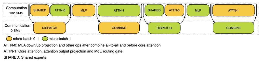
从汇总表可见 Combine 显著小于 Attention,因此官方对 Attention 拆分以 overlap。按如下方式评估 TimeBudget(原文代码保持不变):
dfo=dfs[dfs['TPS_O']>20]
dfo['TimeBudget'] =  dfo['SparseMLA'] + dfo['SharedExpert'] - (dfo['Dispatch']+dfo['Combine'])
print(dfo[['GPU','BatchSize','TimeBudget']].set_index('GPU').to_markdown(floatfmt=".3f"))
结论:H800 通信余量非常小,因此需要 IBGDA;H20 仍存在一定通信余量,但 800G 实例无法满足需求,1.6T 仍有较大余量;而 H20_3e 为保证更大 batchsize 下性能仍需 3.2T 网络,涉及成本权衡。另外,从 timebudget 角度看,网卡等静态延迟影响可忽略。
4. 小结
本文从计算量、显存带宽、网络带宽约束出发,逆向分析了 DeepSeek-R1 在 H800 与 H20 上的推理性能。结论是:
- H800:最佳部署基本对应官方 EP144 方案,分析数据与官方数据一致性较高;并且从 overlap 时间预算看,必须使用 IBGDA 以降低延迟。
- H20:算力约束导致 MLA 计算偏慢,必须用 TP 并行加速;但 TP 过大会因 KVCache 占用使 batchsize 受限。此时 H20-3E(141GB)体现出额外性能收益;对互联带宽评估显示,在 EP 并行实现合理时,1.6Tbps 带宽即可满足需求。
更多相关讨论可到 云栈社区 继续交流。
参考资料
 发表于 2026-1-20 17:24:27
|
查看: 221|
回复: 0
发表于 2026-1-20 17:24:27
|
查看: 221|
回复: 0
