Bi-LSTM双向长短时记忆网络详解：从原理到PyTorch情感分析实战

在序列建模任务中，如何有效捕捉前后文信息一直是个核心问题。传统的单向循环神经网络（RNN）及其变种LSTM，在处理如“我一开始不喜欢，但后来觉得这产品很棒”这类句子时，往往会因只看到前半部分而产生误判。这时，Bi-LSTM（Bidirectional Long Short-Term Memory，双向长短时记忆网络） 的优势便显现出来了。

Bi-LSTM 通过同时结合序列过去与未来的信息，为每个位置提供更全面的上下文编码，在命名实体识别、语义角色标注、情感分析等 自然语言处理 任务中表现出色。

LSTM 核心机制回顾

在深入 Bi-LSTM 之前，有必要简要回顾 LSTM 的原理。LSTM 通过引入精密的门控机制，有效缓解了传统 RNN 的梯度消失或爆炸问题。其核心在于一个名为“细胞状态”（Cell State）的传送带，以及三个负责调控信息的“门”：

• 遗忘门（Forget Gate）：决定从上一个细胞状态 $C_{t-1}$ 中丢弃哪些信息。
• 输入门（Input Gate）：决定当前输入 $x_t$ 和前一时刻隐藏状态 $h_{t-1}$ 中哪些新信息需要存入细胞状态。
• 输出门（Output Gate）：基于当前的细胞状态 $C_t$，决定输出什么样的隐藏状态 $h_t$。

LSTM 前向传播公式

给定输入序列 $\\{x_1, x_2, ..., x_T\\}$，对于第 $t$ 个时间步，其计算过程如下：

1. 遗忘门：$f_t = \\sigma(W_f \\cdot [h_{t-1}, x_t] + b_f)$
2. 输入门：$i_t = \\sigma(W_i \\cdot [h_{t-1}, x_t] + b_i)$
3. 候选记忆：$\\tilde{C_t} = \\tanh(W_C \\cdot [h_{t-1}, x_t] + b_C)$
4. 更新细胞状态：$C_t = f_t \\odot C_{t-1} + i_t \\odot \\tilde{C_t}$
5. 输出门：$o_t = \\sigma(W_o \\cdot [h_{t-1}, x_t] + b_o)$
6. 当前隐藏状态：$h_t = o_t \\odot \\tanh(C_t)$

其中，$\\sigma$ 表示 Sigmoid 激活函数，$\\odot$ 表示逐元素相乘，$[h_{t-1}, x_t]$ 表示向量拼接。

Bi-LSTM 结构剖析

Bi-LSTM 的核心思想简单而强大：使用两个独立的 LSTM 层分别从正向和反向处理输入序列。

• 正向 LSTM：沿时间步 $1 \\rightarrow T$ 顺序处理输入，生成隐藏状态序列 $\\overrightarrow{h_1}, \\overrightarrow{h_2}, ..., \\overrightarrow{h_T}$，它编码了当前位置及之前的所有上文信息。
• 反向 LSTM：沿时间步 $T \\rightarrow 1$ 逆序处理输入，生成隐藏状态序列 $\\overleftarrow{h_1}, \\overleftarrow{h_2}, ..., \\overleftarrow{h_T}$，它编码了当前位置及之后的所有下文信息。

对于最终在时间步 $t$ 的输出，Bi-LSTM 将正向和反向的隐藏状态进行拼接：

这个拼接后的向量 $h_t$ 同时蕴含了该词（或时间步）左右两侧的完整上下文信息。

一个完整的 PyTorch 实战案例：情感分析

理论需要实践来验证。下面我们将构建一个基于 Bi-LSTM 的情感分类模型，任务是将英文短句分类为“积极”、“消极”或“中性”。

步骤 1：构建虚拟数据集

为了便于演示，我们直接生成一个包含三类情感短语的小型数据集。

import random

def generate_sample():
    positive_phrases = [
        "I love this product", "This is amazing", "Absolutely wonderful",
        "I am very satisfied", "Highly recommend it"
    ]
    negative_phrases = [
        "I hate this", "Very disappointed", "Absolutely terrible",
        "Worst experience ever", "I want a refund"
    ]
    neutral_phrases = [
        "It arrived today", "The box is blue", "It is okay",
        "Not sure yet", "Just received it"
    ]

    data = []
    for phrase in positive_phrases:
        data.append((phrase.split(), 0))  # label 0 = positive
    for phrase in negative_phrases:
        data.append((phrase.split(), 1))  # label 1 = negative
    for phrase in neutral_phrases:
        data.append((phrase.split(), 2))  # label 2 = neutral

    random.shuffle(data)
    return data

步骤 2：数据预处理与模型定义

接下来，我们将文本转换为模型可读的索引序列，并定义 Bi-LSTM 模型。

import torch
import torch.nn as nn
import torch.optim as optim
from torch.utils.data import DataLoader, Dataset
import numpy as np

# 生成数据并构建词汇表
data = generate_sample()
vocab = {word for sent, _ in data for word in sent}
word2idx = {w: i+1 for i, w in enumerate(sorted(vocab))}
word2idx['<PAD>'] = 0
vocab_size = len(word2idx)
num_classes = 3

# 数据编码函数
def encode(sample):
    words, label = sample
    max_len = 6
    x = [word2idx.get(w, 0) for w in words]
    x += [0] * (max_len - len(x))
    return x[:max_len], label

encoded = [encode(s) for s in data]
X, y = zip(*encoded)
X = torch.tensor(X, dtype=torch.long)
y = torch.tensor(y, dtype=torch.long)

# 自定义 Dataset
class SentimentDataset(Dataset):
    def __init__(self, X, y):
        self.X = X
        self.y = y
    def __len__(self):
        return len(self.X)
    def __getitem__(self, idx):
        return self.X[idx], self.y[idx]

dataset = SentimentDataset(X, y)
train_loader = DataLoader(dataset, batch_size=4, shuffle=True)

# 定义 Bi-LSTM 模型
class BiLSTMModel(nn.Module):
    def __init__(self, vocab_size, embed_dim, hidden_dim, output_dim):
        super().__init__()
        self.embed = nn.Embedding(vocab_size, embed_dim, padding_idx=0)
        # 关键：设置 bidirectional=True
        self.lstm = nn.LSTM(embed_dim, hidden_dim, bidirectional=True, batch_first=True)
        # 因为是双向，全连接层输入维度是 hidden_dim * 2
        self.fc = nn.Linear(hidden_dim * 2, output_dim)

    def forward(self, x):
        x = self.embed(x)  # [batch, seq_len, embed_dim]
        # LSTM输出取最后时刻的正向和反向隐藏状态
        _, (h_n, _) = self.lstm(x)  # h_n shape: [2*num_layers, batch, hidden_dim]
        # 拼接正向和反向的最终状态
        h_cat = torch.cat((h_n[0], h_n[1]), dim=1)  # [batch, hidden_dim*2]
        out = self.fc(h_cat)
        return out

# 实例化模型、损失函数和优化器
model = BiLSTMModel(vocab_size, 50, 64, num_classes)
criterion = nn.CrossEntropyLoss()
optimizer = optim.Adam(model.parameters(), lr=0.005)

步骤 3：训练模型

我们进行一个简单的训练循环，并记录损失和准确率。

losses = []
accuracies = []
from sklearn.metrics import accuracy_score

for epoch in range(20):
    model.train()
    all_preds, all_labels = [], []
    epoch_loss = 0.0
    for batch_x, batch_y in train_loader:
        optimizer.zero_grad()
        output = model(batch_x)
        loss = criterion(output, batch_y)
        loss.backward()
        optimizer.step()
        epoch_loss += loss.item()
        all_preds += output.argmax(dim=1).tolist()
        all_labels += batch_y.tolist()

    acc = accuracy_score(all_labels, all_preds)
    losses.append(epoch_loss / len(train_loader))
    accuracies.append(acc)
    print(f"Epoch {epoch+1}: Loss = {losses[-1]:.4f}, Accuracy = {acc:.2f}")

步骤 4：模型性能可视化

训练完成后，通过多维度图表来分析模型表现。

import matplotlib.pyplot as plt
from sklearn.metrics import confusion_matrix
import seaborn as sns

fig, axs = plt.subplots(2, 2, figsize=(14, 10))
plt.subplots_adjust(hspace=0.4)

# 图1：训练损失曲线
axs[0, 0].plot(losses, color='crimson', marker='o', linewidth=2)
axs[0, 0].set_title("Training Loss", fontsize=14)
axs[0, 0].set_xlabel("Epoch")
axs[0, 0].set_ylabel("Loss")

# 图2：训练准确率曲线
axs[0, 1].plot(accuracies, color='royalblue', marker='s', linewidth=2)
axs[0, 1].set_title("Training Accuracy", fontsize=14)
axs[0, 1].set_xlabel("Epoch")
axs[0, 1].set_ylabel("Accuracy")

# 图3：混淆矩阵
model.eval()
with torch.no_grad():
    y_true = y.tolist()
    y_pred = model(X).argmax(dim=1).tolist()

cm = confusion_matrix(y_true, y_pred)
sns.heatmap(cm, annot=True, fmt="d", cmap="YlGnBu", ax=axs[1, 0])
axs[1, 0].set_title("Confusion Matrix", fontsize=14)
axs[1, 0].set_xlabel("Predicted")
axs[1, 0].set_ylabel("Actual")

# 图4：预测与实际分布对比
pred_counts = np.bincount(y_pred, minlength=3)
true_counts = np.bincount(y_true, minlength=3)
bar_width = 0.35
index = np.arange(3)

axs[1, 1].bar(index, true_counts, bar_width, label='True', color='limegreen')
axs[1, 1].bar(index + bar_width, pred_counts, bar_width, label='Pred', color='orange')
axs[1, 1].set_title("Prediction vs Actual Distribution", fontsize=14)
axs[1, 1].set_xticks(index + bar_width / 2)
axs[1, 1].set_xticklabels(["Positive", "Negative", "Neutral"])
axs[1, 1].legend()

plt.suptitle("Bi-LSTM Performance Analysis", fontsize=16)
plt.show()

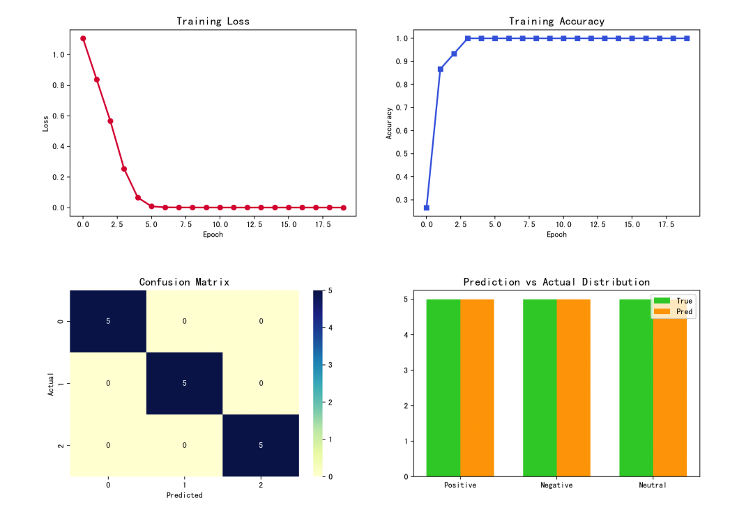
从上图的四联分析图可以看出，在这个小型数据集上，Bi-LSTM模型迅速收敛，训练损失稳步下降，准确率很快达到1.0。混淆矩阵显示所有样本均被正确分类，预测分布与实际分布完全一致，证明了模型的有效性。

技术总结与思考

Bi-LSTM 的核心优势在于其双向上下文建模能力。相比于单向 LSTM，它在处理需要综合前后文信息才能做出准确判断的任务时，具有天然的优势。例如，在“这个苹果很好吃，但那个不行”的句子中，要判断“苹果”的情感，反向的“不行”信息至关重要。

当然，Bi-LSTM 并非没有代价。其计算量约为单向 LSTM 的两倍，且在实时流式处理场景（如语音识别）中，反向计算需要等待完整序列，可能引入延迟。随着 Transformer 和基于自注意力机制模型的兴起，它们在长序列建模上展现出更强的能力，但 Bi-LSTM 因其结构清晰、在短文本任务上效果稳定，仍然是 深度学习 序列建模工具包中不可或缺的一员，特别是在计算资源有限或需要模型轻量化的场景下。

本文从数学原理、结构推理到 PyTorch 实战，系统解析了 Bi-LSTM。希望这份详细的梳理能帮助你更扎实地掌握这一经典模型。如果你想探索更多机器学习和 算法/数据结构 相关内容，欢迎到 云栈社区 与更多开发者交流讨论。