昨天写了 ADI 的信号发生单元 ADMX-1001,里面还有很多细节没有展开。今天这篇文章主要来说明 DPD 算法的一些实现细节,内容基于专利和信号链的理解整理而成。如果还没有看过前一篇,可以先了解一下背景:ADMX1001低失真信号发生器:钱包空了也变强了~
−130 dBc 到底是什么?
这台仪器的设计复杂度相当高,核心指标就是下面这张图里的 THD:

24 bit 的 ADC 是可以给出这个值的:
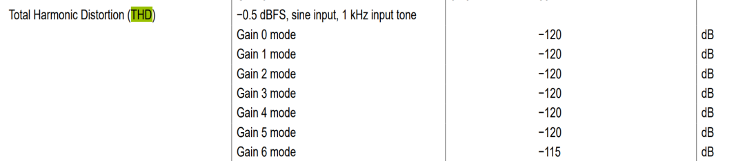
这里的 −130 dBc 是输出正弦波的总谐波失真 THD 相对于基波的比值,c 表示 carrier,也就是以基波为参考,而不是相对于满量程。ADI 手册里对 THD 的定义如下:
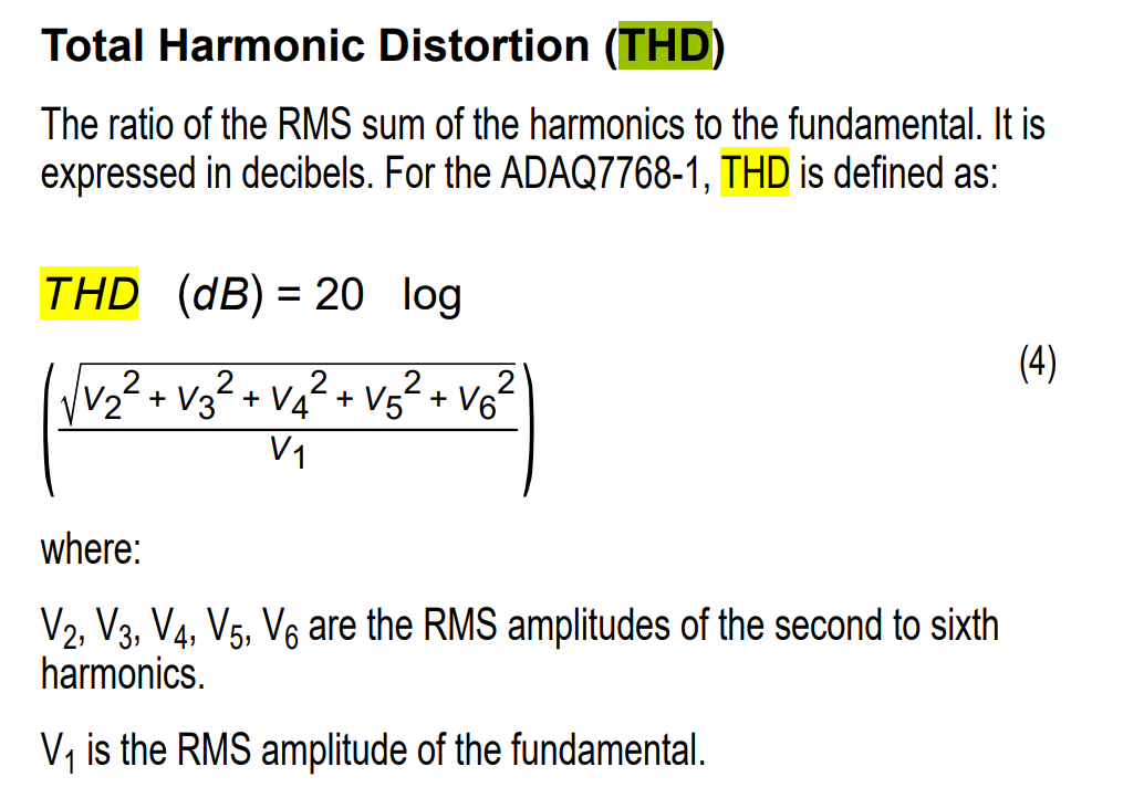
计算方式通常为:
$$\text{THD(dB)} = 20\log_{10}\left(\frac{\sqrt{V_2^2 + V_3^2 + V_4^2 + V_5^2 + V_6^2}}{V_1}\right)$$
其中:
- $V_1$:基波 RMS 电压
- $V_2, V_3, \ldots$:二次、三次及更高次谐波的 RMS 电压
−130 dBc 对应的谐波电压比例为:
$$10^{-130/20} \approx 3.16 \times 10^{-7}$$
也就是约 0.316 ppm。
| 基波幅度 |
−130 dBc 对应的总谐波 RMS |
| 1 V RMS |
0.316 µV RMS |
| 2 V RMS |
0.632 µV RMS |
| 3 V RMS |
0.949 µV RMS |
例如输出 2 V RMS、1 kHz 正弦时,二次及以上所有谐波平方和的 RMS 只有约 0.632 µV。
这个指标有什么用?
它表示信号源本身有多“纯”。如果用信号源测试 ADC、音频编解码器或放大器:
测得的失真 ≈ 信号源失真 + DUT 失真 + 测量系统失真
假设被测 ADC 的 THD 是 −110 dBc,而信号源只有 −100 dBc,那么最后主要测到的是信号源,不是 ADC。通常希望激励源比 DUT 好至少 10~15 dB:
| 被测设备 THD |
建议激励源 THD |
| −90 dBc |
≤ −105 dBc |
| −100 dBc |
≤ −115 dBc |
| −110 dBc |
≤ −125 dBc |
| −115 dBc |
接近 −130 dBc |
所以 −130 dBc 主要服务于高端音频 ADC、精密 ADC 和超低失真放大器测试。它不是所有应用都必须达到的指标。另外,−130 dBc THD 不等于整个系统拥有 130 dB SNR;它只描述谐波,不包括宽带噪声、电源杂散和时钟杂散。
ADMX1001 差分感测与数字预失真专利算法分析
说明一下,这里研究的是 ADI ADMX1001/ADMX1002 的单音数字预失真(DPD)机制。算法仿真属于行为级别,实际使用需要深入到固件级别。
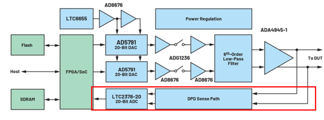
专利的分析
最直接描述幅度差分、相位分箱、波形重构和相位相关修正的专利是 US11018681B1。固定电压跨度、测量穿越时间的早期时间差分方法,主要对应 US9998133B2 及其同族/前序专利。感兴趣的话可以在谷歌专利中查到原文。
ADI 的“差分时间与幅度感测”是对一组互补专利方法的产品化概括。这些方法没有让反馈 ADC 本身变得更线性;只是把困难的全量程绝对电压测量转换成局部的电压差或时间差测量,再通过相位分箱、重复平均、周期积分和频谱分析重建失真。
当前 Python 行为模型中,补偿前 THD 为 −86.88 dBc,补偿后的最佳 THD 为 −130.83 dBc,改善约 43.95 dB。
ADI 官方系统文档对 ADMX1001/ADMX1002 的描述是:DPD 不需要外部参考输入;使用获得专利的差分时间和幅度感测方法;针对单音正弦波进行自感测修正;DPD 打开时信号范围最高约为 20 kHz;1 kHz 下典型 THD 可达到约 −130 dBc。
另外,ADI 技术文章进一步披露了算法框架:在校准阶段产生一个单频正弦波;DPD sense path 在 ADC 前改善针对这种信号的测量线性;采集波形的多个数字化片段;在数字域重建信号;将重建结果与数学模型比较;提取修正参数并用于新的正弦波生成;反复迭代以降低随机误差;找到最佳修正后停止并保存参数。
(另外还有一些专利的转让,最早可能是 Ateeda Ltd. 的,不过这不是重点。)
这些专利要解决的根本问题
用什么测量一个比反馈 ADC 更线性的 DAC?
设 DAC 的目标输出是一个理想正弦波,DAC 和输出模拟链路会产生非线性误差,反馈 ADC 又具有自身的增益、失调、INL 和噪声。简化后可写成:
$$z[k] = f\left(y[k]\right) + n[k]$$
直接对反馈 ADC 数据做 FFT,得到的第 $n$ 次谐波近似为 DAC 失真与 ADC 失真的混合结果。于是无法判断谐波究竟来自 DAC 还是反馈 ADC。若把反馈 ADC 自身的失真当成 DAC 失真并进行反向补偿,校准可能越调越差。
传统直接测量面临的限制
反馈 ADC 的全量程 INL 可能不优于输出 DAC;ADC 失调、增益误差和低频漂移进入测量结果;缓冲器、衰减器和重构滤波器也会产生失真;−120~−130 dBc 的谐波远低于主信号;使用更好的外部分析仪违背小型化、自校准和低成本目标;若测试 ADC,测试源必须明显优于被测 ADC,形成测量能力的循环依赖。
专利的解决思路不是制造一个“完美 ADC”,而是改变需要测量的量。
共通思想:从绝对测量改为局部差分测量
两组专利都把问题从:
当前点的绝对电压是多少?
转换为:
一个很短的局部片段改变了多少电压,或者跨过固定电压用了多少时间?
局部差分对应波形的导数。对于理想正弦:
$$\frac{dy}{d\phi} = A\cos(\phi)$$
只要知道片段所在相位,就知道理想正弦在该位置应有的局部变化。实际变化与理想变化之间的差异,包含了非线性失真的信息。
时间差分感测:固定电压差,测量时间差
时间差分方法主要对应 US9998133B2。
基本测量
设置两个固定阈值,固定电压跨度为 $\Delta V$,测量局部波形从低阈值移动到高阈值所需的时间 $\Delta t$。局部斜率估计为:
$$\widehat{\frac{dy}{d\phi}} \approx \frac{\Delta V}{\Delta t}$$
下降沿需要附加斜率符号。理想正弦在该相位的斜率为 $A\cos(\phi)$,局部斜率误差可以反映波形非理想程度。
重基准的作用
原始正弦波可能跨越很大的电压范围。专利利用电容、模拟开关和参考电平,把不同位置的小片段搬到同一对比较器阈值附近:
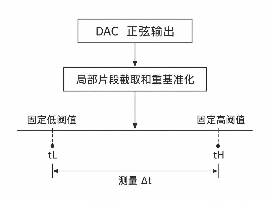
即使原始片段分别位于正电压、零点附近或负电压,比较器始终在近似相同的电压条件下工作。
它降低了哪些误差要求?
不要求知道每个片段的绝对电压;固定比较器失调在重复差分中表现为近似公共误差;测量重点变成阈值间隔的稳定性和时间测量分辨率;可以利用高速计数器或 TDC 精确测量 $\Delta t$;同一相位的重复样本可以平均,降低随机抖动;无需反馈 ADC 在整个输出范围都比 DAC 更线性。
但问题是正弦顶部和底部的斜率趋近于零,穿越时间变长且条件数恶化;比较器传播延迟可能依赖输入斜率;时间基准抖动直接进入斜率估计;需要在转折点附近插值或采用额外的斜坡测试;重基准开关会带来电荷注入和建立时间问题。
幅度差分感测:固定时间差,测量电压差
幅度差分方法主要对应 US11018681B1。
两点局部差分
在同一局部片段内选择两个已知相位,测得局部电压差 $\Delta V$。对于理想正弦:
$$\Delta V_{\text{ideal}} = A\left[\sin(\phi_2) - \sin(\phi_1)\right]$$
因此可得到局部等效幅度:
$$\hat{A} = \frac{\Delta V}{\sin(\phi_2) - \sin(\phi_1)}$$
理想正弦的所有局部幅度估计应当相同。如果 $\hat{A}$ 随相位变化,说明输出不是理想正弦,存在相位相关非线性。
为什么重新基准化很重要?
假设 DAC 输出范围为大幅值摆幅,直接测量要求 ADC 在整个范围内都具有极高线性。局部切片和重基准后,每个片段可以被搬到类似的小范围区间。ADC 实际需要测量的主要信息只是局部差分值。因此系统更依赖 ADC 在小范围内的局部线性、短期重复性和噪声,而不是完整静态传输曲线的全量程 INL。
固定 ADC 失调在两点相减时消除;ADC 增益误差主要成为整体比例误差;缓慢漂移在短时间片段内近似公共模;全量程非线性不会逐点直接映射到重构波形;局部差值可以跨多个周期重复测量并平均;切片频率可以选择为使片段幅度落入 ADC 的高线性局部区域。
需要强调:这种方法不是数学上完全消除 ADC INL。ADC 的局部曲率、动态非线性、采样电荷注入和噪声仍然存在,只是误差敏感性被重新分配了。
多周期采集、相位分箱和平均
单次差分样本仍然包含噪声,因此专利在多个周期内采集不同相位位置的片段:
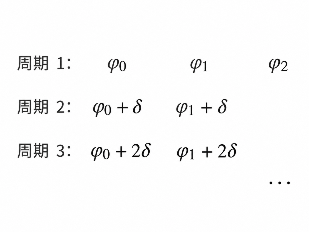
把样本按照相位放入第 $k$ 个相位箱:
$$q_k = \text{median}\left(q_i\right)$$
其中 $q_i$ 可以是局部幅度、局部电压差或局部导数估计。每个相位箱取均值、中位数或其他中心趋势。对于独立随机噪声,使用均值时标准差近似按 $1/\sqrt{N}$ 的规律下降。当前 Python 模型使用中位数,以模拟对开关瞬态和异常样本的稳健抑制。
从局部差分重建周期波形
周期前向差分
令离散周期波形为 $y[k]$,相邻相位箱差分为:
$$d[k] = y[k+1] - y[k]$$
直接累加可以重建波形,但噪声会产生累计漂移,而且差分测量丢失 DC 信息。
Python 中采用的周期最小二乘积分
为了避免把闭合误差累积成斜坡,程序在频域反演周期前向差分算子。第 $m$ 个频率点的差分传递函数为:
$$H_m = e^{j2\pi m/N} - 1$$
因此对于所有非 DC 频率:
$$\hat{Y}_m = \frac{D_m}{H_m}$$
再做逆 FFT 即得到零均值重构波形。这样会把周期闭合误差分散到整个周期,而不是在末端形成明显跳变。
恢复基波
差分操作丢失 DC,并且实际校准主要关注失真而不是绝对偏置。程序通过最小二乘拟合获得基波幅度、相位和 DC,再将基波分量与差分重构结果组合。
从重构波形提取失真
从重构波形中减去最佳拟合基波:
$$e[k] = y_{\text{recon}}[k] - y_{\text{fund}}[k]$$
对误差做离散傅里叶变换,获得各次谐波的复数幅度和相位。THD 定义为:
$$\text{THD(dBc)} = 20\log_{10}\left(\frac{\sqrt{\sum_{n=2}^{H} |E_n|^2}}{|E_1|}\right)$$
数字预失真迭代
设第 $i$ 次迭代的数字驱动波形为 $x_i(\phi)$,由差分感测重构的谐波失真为 $e_i(\phi)$。程序仅保留第 2~第 9 次谐波:
$$x_{i+1} = x_i - \mu \cdot \frac{e_i^{(2..9)}}{G}$$
其中 $\mu$ 是学习率,$G$ 是输出路径的近似增益。基波和 DC 不参与本次谐波 DPD 更新。
每次更新后重新通过非线性 DAC 模型、重新感测和重构。若感测到的 THD 改善小于设定阈值,算法停止,并保留前一个最佳波形。这对应 ADI 文章中“找到最佳修正后停止并保存参数”的公开描述。
Python 仿真模型
一般不太讲程序,不过考虑到这个是行为仿真,也可以放出来。先把依赖库装好。
非线性 DAC/输出路径
模型为无记忆多项式:
$$y = Gx + a_2x^2 + a_3x^3 + a_5x^5$$
默认参数:
| 参数 |
数值 |
| 增益 $G$ |
1.0 |
| 二次项 $a_2$ |
$6.0 \times 10^{-5}$ |
| 三次项 $a_3$ |
$2.0 \times 10^{-4}$ |
| 五次项 $a_5$ |
$5.0 \times 10^{-5}$ |
| 正弦峰值 |
0.80 |
这是行为模型,不包含 DAC 量化、建立时间、去毛刺开关和重构滤波器;那些效应可在后续模型中叠加。
不理想反馈 ADC
反馈 ADC 模型为:
$$y = b_0 + b_1x + b_2x^2 + b_3x^3$$
默认参数:
| 参数 |
数值 |
| 增益 $b_1$ |
1.0 |
| 失调 $b_0$ |
30 µV |
| 二次项 $b_2$ |
$1.2 \times 10^{-4}$ |
| 三次项 $b_3$ |
$-1.6 \times 10^{-4}$ |
| 每次 ADC 测量噪声 |
1.2 µV RMS |
这些数值被有意设置为使直接反馈测量明显受到 ADC 自身失真污染,从而可以观察差分重基准方法的作用。
差分采样和迭代参数
| 参数 |
默认值 |
| 每周期相位箱数 |
256 |
| 每相位重复次数 |
401 |
| 重基准中心误差 |
30 µV RMS |
| 时间感测固定电压跨度 |
50 µV(归一化模型) |
| 时间抖动 |
0.03 ppm/cycle |
| 最大迭代次数 |
8 |
| 学习率 |
0.72 |
| 修正谐波 |
第 2~第 9 次 |
| 最小继续改善量 |
0.5 dB |
| 随机种子 |
1001/1002/1003 |
幅度感测、时间感测和 DPD 使用相互独立的确定性随机数流,改变时间感测参数不会意外改变 DPD 的噪声序列。
函数对应关系
| Python 函数 |
作用 |
Plant.__call__() |
非线性 DAC/模拟路径 |
FeedbackADC.noiseless() |
反馈 ADC 静态非线性 |
amplitude_differential_sense() |
重基准后的局部幅度差、相位分箱和重构 |
temporal_differential_sense() |
固定电压跨度的阈值穿越时间行为模型 |
invert_periodic_forward_difference() |
周期差分的频域最小二乘积分 |
best_fit_fundamental() |
最小二乘拟合 DC、正弦和余弦基波 |
harmonic_only() |
选择需要修正的谐波 |
learn_predistortion() |
迭代 DPD 和最佳结果保留 |
thd_db() |
计算 THD,单位 dBc |
write_plots() |
每项结果分别输出独立 PNG |
算结果
结果由当前默认参数和固定随机种子实际运行得到:
Patent-inspired differential DPD simulation
Before DPD THD:                    -86.88 dBc
After DPD THD:                    -130.83 dBc
Improvement:                        43.95 dB
Direct ADC distortion error:       30.780 uV RMS
Amplitude reconstruction error:     0.395 uV RMS
Temporal reconstruction error:      7.319 uV RMS
Final sensed THD:                 -132.99 dBc
可以看到如果直接使用不理想 ADC 测量时,ADC 自身造成的失真误差为 30.780 µV RMS;使用局部重基准幅度差分重构误差降低到 0.395 µV RMS;教学级时间差分模型重构误差为 7.319 µV RMS;DPD 将实际输出 THD 从 −86.88 dBc 改善到 −130.83 dBc;最终差分感测估计为 −132.99 dBc,与实际值存在约 2.16 dB 差异,体现有限噪声和估计偏差。
每次迭代结果
| 迭代 |
差分感测估计 THD (dBc) |
实际 DAC 输出 THD (dBc) |
| 0 |
−92.907566 |
−86.878752 |
| 1 |
−104.156462 |
−97.917058 |
| 2 |
−113.410084 |
−108.391209 |
| 3 |
−124.691140 |
−121.757438 |
| 4 |
−132.986337 |
−130.829787 |
| 5 |
−133.111910 |
−129.649795 |
迭代 5 的感测估计只比迭代 4 改善约 0.126 dB,低于默认 0.5 dB 的继续改善阈值,因此算法停止并保留迭代 4 的驱动波形。这样可以避免在噪声地板附近继续追逐随机测量误差。
各次谐波计算值
| 谐波 |
补偿前 (dBc) |
补偿后最佳结果 (dBc) |
| 1 |
0.000000 |
0.000000 |
| 2 |
−92.396720 |
−145.143726 |
| 3 |
−88.314320 |
−142.195989 |
| 4 |
−331.952056 |
−137.842493 |
| 5 |
−117.856746 |
−133.225936 |
| 6 |
−334.656739 |
−145.133199 |
| 7 |
−343.523615 |
−144.717908 |
| 8 |
−342.635495 |
−145.313899 |
| 9 |
−339.610071 |
−159.136687 |
非常低的补偿前偶次/高次谐波,例如 −330 dBc 以下,是理想浮点多项式模型中理论为零或极小的项,不代表真实硬件可以达到该数值。实际系统会受到量化噪声、时钟抖动、热噪声、开关电荷注入、滤波器失真和数值噪声限制。
预失真和最终残差
| 指标 |
数值 |
| 注入预失真 RMS |
25.637832 µV |
| 注入预失真峰值 |
50.671242 µV |
| 补偿后去基波残差 RMS |
0.162605 µV |
| 补偿后去基波残差峰值 |
0.333469 µV |
这些数值以归一化 1 V 标度表达;说明微伏量级的数字波形修正可以抵消多项式模型产生的主要谐波,但不能直接当作 ADMX1001 硬件上的实测电压。
非线性 DAC 输出
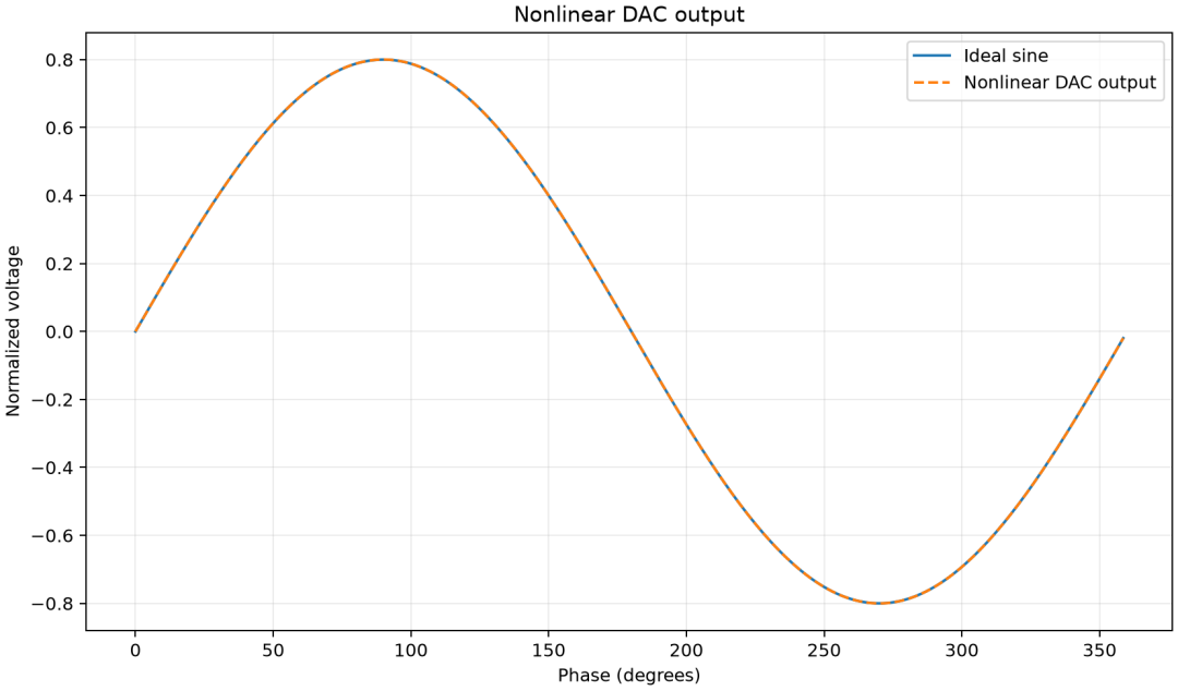
理想正弦与非线性 DAC 输出在正常比例下几乎重合,说明仅看时域主波形很难观察微小谐波失真。
直接 ADC 测量的歧义
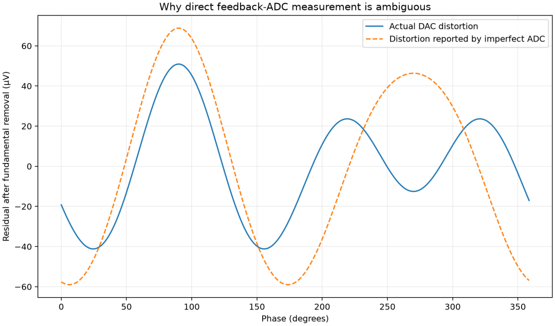
去掉最佳拟合基波后,可以看到反馈 ADC 报告的失真与 DAC 实际失真明显不同;直接测量会把 ADC 的非线性混入 DAC 误差。
幅度差分局部片段
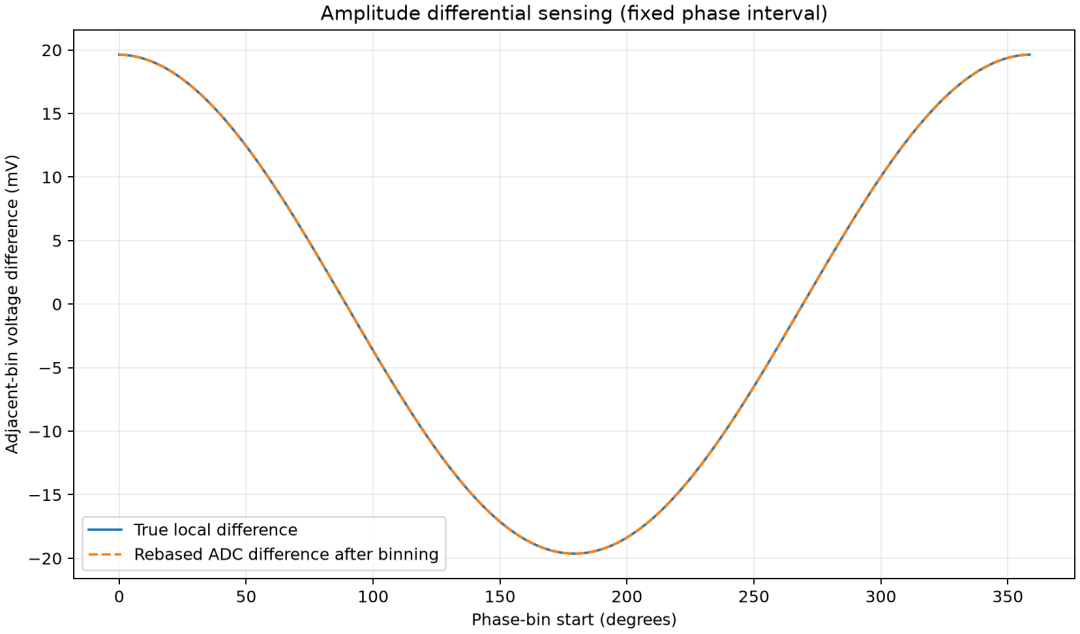
图中比较真实相邻相位电压差与局部重基准、重复分箱后得到的差值。两条曲线应基本重合。
时间差分局部斜率
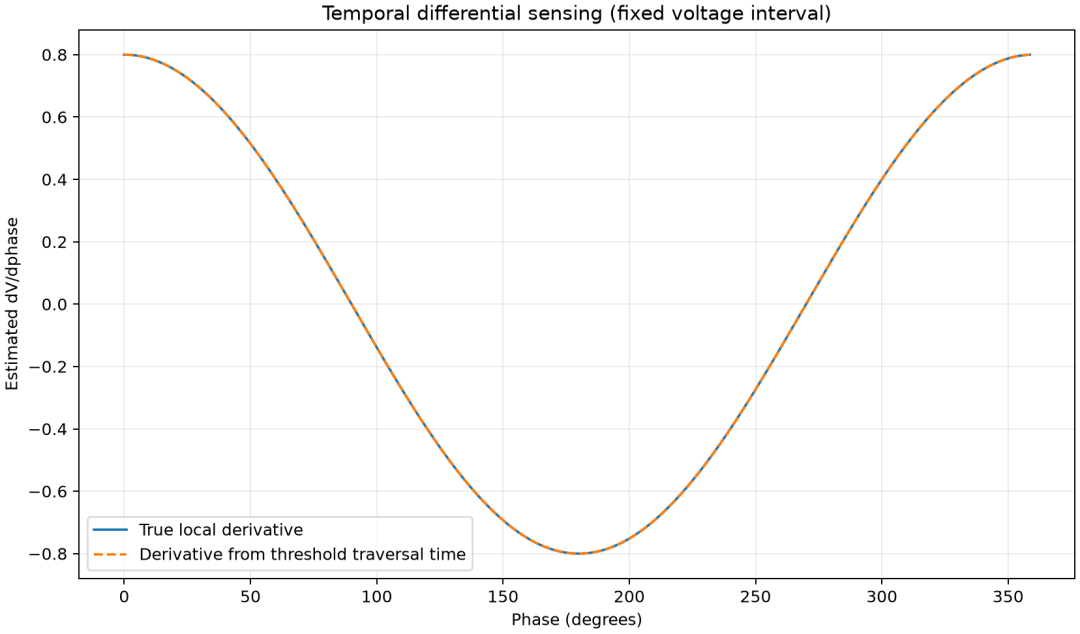
图中比较真实导数和由固定电压跨度穿越时间估计的导数;转折点附近因为斜率接近零,需要周期插值,误差大于幅度差分模型。
差分重构的失真
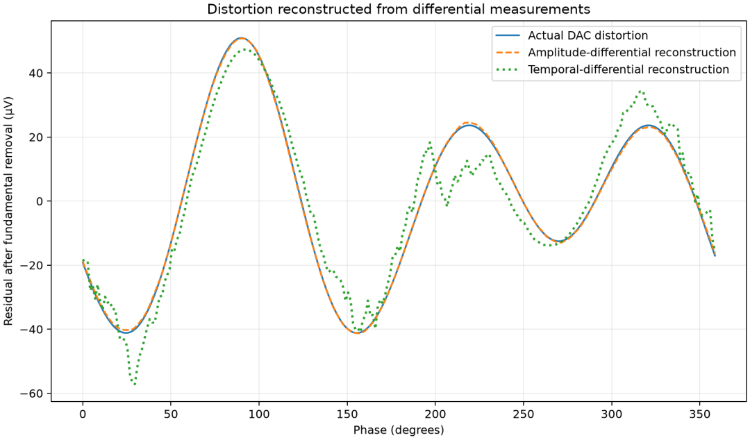
幅度差分重构几乎覆盖真实 DAC 失真;时间差分的教学模型在转折点和插值区域误差更明显。
补偿前后谐波
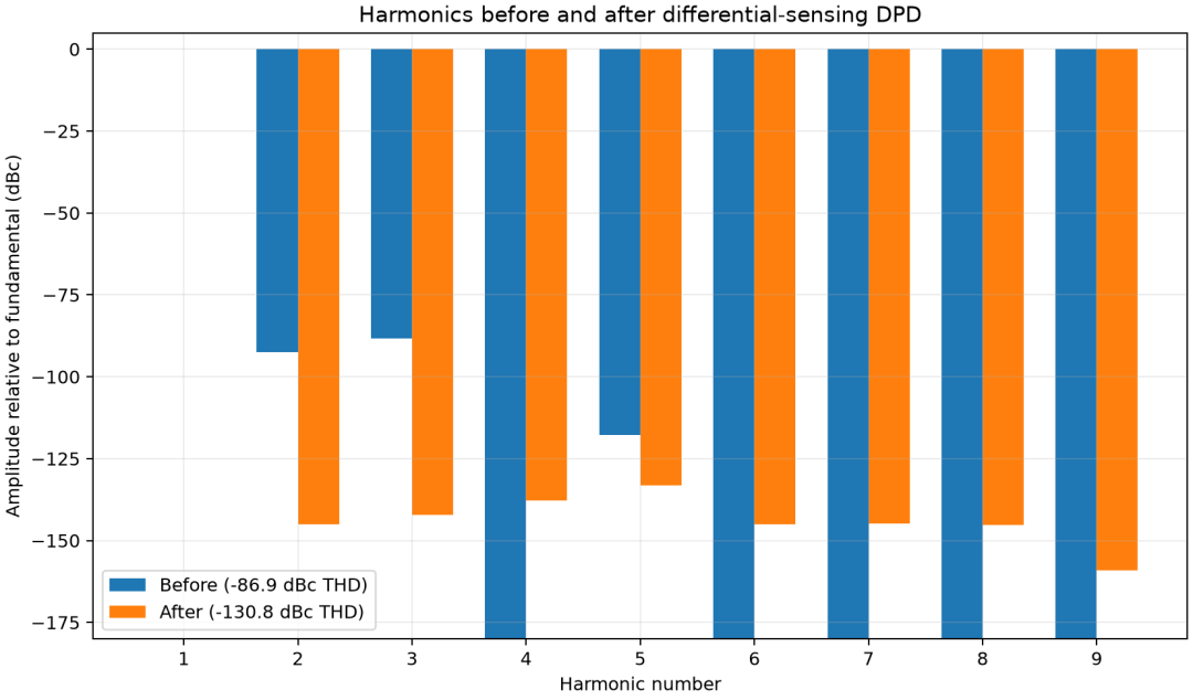
主要二次、三次和五次谐波被显著压低,综合 THD 从 −86.88 dBc 降至 −130.83 dBc。
DPD 收敛过程
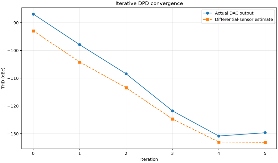
迭代初期快速收敛;进入噪声限制区后,估计值和真实值可能不再同步改善,因此需要停止条件和最佳波形回退。
注入预失真和最终残差
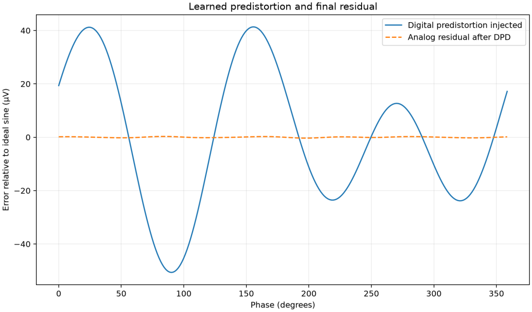
数字端注入的预失真与模拟路径产生的非线性方向相反,最终模拟输出只保留很小的残差。
如何理解“绕开反馈 ADC 全量程 INL”?
“绕开”不应理解为反馈 ADC 的非线性完全消失。更准确的表述是:
差分重基准方法把对反馈 ADC 的要求,从整个输入范围上的绝对传输精度,转化为小局部范围内的差分线性、重复性、短期稳定性和噪声性能。
能够抑制或弱化的因素包括:绝对失调、部分增益误差、缓慢公共漂移、大范围静态传输曲线弯曲、非相干随机噪声。
小结
这组专利的核心是一种测量架构转换:在工程上用一个并不明显优于 DAC 的反馈 ADC,把直接测量 DAC 全量程微小失真,转换为切分周期波形 → 重基准到局部小范围 → 测 ΔV 或 Δt → 按相位重复分箱 → 重建导数/波形 → 提取谐波 → 生成反向校正 → 迭代并保存最佳结果。
只让测量通道完成它最擅长的局部差分测量,再利用周期性、相位知识、重复平均和数字重构获得高精度失真估计,最后通过迭代预失真提高正弦输出纯度。
行为级模型差了很多非理想因素,实际效果需要写代码实测验证,散会!
完整代码
from __future__ import annotations

import argparse
import csv
from dataclasses import dataclass
from pathlib import Path
import matplotlib.pyplot as plt
import numpy as np

EPSILON = np.finfo(float).tiny

@dataclass(frozen=True)
class Plant:
    """Memoryless DAC/output-path polynomial."""

    gain: float = 1.0
    a2: float = 6.0e-5
    a3: float = 2.0e-4
    a5: float = 5.0e-5

    def __call__(self, code: np.ndarray) -> np.ndarray:
        return (
            self.gain * code
            + self.a2 * code**2
            + self.a3 * code**3
            + self.a5 * code**5
        )

@dataclass(frozen=True)
class FeedbackADC:
    """Deliberately imperfect feedback ADC transfer characteristic."""

    gain: float = 1.0
    offset: float = 30.0e-6
    b2: float = 1.2e-4
    b3: float = -1.6e-4

    def noiseless(self, voltage: np.ndarray) -> np.ndarray:
        return (
            self.offset
            + self.gain * voltage
            + self.b2 * voltage**2
            + self.b3 * voltage**3
        )

def best_fit_fundamental(signal: np.ndarray, phase: np.ndarray) -> np.ndarray:
    """Return the least-squares DC + fundamental component of a waveform."""
    design = np.column_stack((np.sin(phase), np.cos(phase), np.ones_like(phase)))
    coefficients, *_ = np.linalg.lstsq(design, signal, rcond=None)
    return design @ coefficients

def remove_fundamental(signal: np.ndarray, phase: np.ndarray) -> np.ndarray:
    return signal - best_fit_fundamental(signal, phase)

def harmonic_complex(signal: np.ndarray, maximum_harmonic: int) -> np.ndarray:
    """Complex FFT coefficients for harmonics 0..maximum_harmonic."""
    spectrum = np.fft.rfft(signal) / signal.size
    return spectrum[: maximum_harmonic + 1]

def harmonic_levels_db(signal: np.ndarray, maximum_harmonic: int) -> np.ndarray:
    coefficients = harmonic_complex(signal, maximum_harmonic)
    peak = 2.0 * np.abs(coefficients)
    return 20.0 * np.log10(np.maximum(peak[1:] / peak[1], EPSILON))

def thd_db(signal: np.ndarray, maximum_harmonic: int) -> float:
    coefficients = harmonic_complex(signal, maximum_harmonic)
    peak = 2.0 * np.abs(coefficients)
    ratio = np.sqrt(np.sum(peak[2:] ** 2)) / peak[1]
    return 20.0 * np.log10(max(ratio, EPSILON))

def harmonic_only(
    signal: np.ndarray,
    first_harmonic: int,
    last_harmonic: int,
) -> np.ndarray:
    """Keep selected coherent harmonics and reject DC/fundamental/noise."""
    spectrum = np.fft.rfft(signal)
    selected = np.zeros_like(spectrum)
    selected[first_harmonic : last_harmonic + 1] = spectrum[
        first_harmonic : last_harmonic + 1
    ]
    return np.fft.irfft(selected, n=signal.size)

def invert_periodic_forward_difference(difference: np.ndarray) -> np.ndarray:
    """Least-squares periodic integration with the unknown DC set to zero.

    For d[k] = y[k+1] - y[k], the Fourier-domain transfer function is
    exp(j*2*pi*m/N)-1. Inverting every non-DC bin automatically distributes
    closure error instead of accumulating it as a ramp.
    """
    count = difference.size
    bins = np.arange(count // 2 + 1)
    transfer = np.exp(2j * np.pi * bins / count) - 1.0
    transformed = np.fft.rfft(difference)
    reconstructed = np.zeros_like(transformed)
    reconstructed[1:] = transformed[1:] / transfer[1:]
    return np.fft.irfft(reconstructed, n=count)

def amplitude_differential_sense(
    analog_output: np.ndarray,
    adc: FeedbackADC,
    repeats: int,
    noise_rms: float,
    rebase_error_rms: float,
    rng: np.random.Generator,
) -> tuple[np.ndarray, np.ndarray, np.ndarray]:
    """Reconstruct a waveform from locally rebased amplitude differences.

    Each phase bin is observed ``repeats`` times. The two endpoints are
    translated into the same small ADC region, so full-scale ADC INL is not
    directly mapped onto the DAC waveform.
    """
    true_difference = np.roll(analog_output, -1) - analog_output
    count = analog_output.size
    measured = np.empty((repeats, count))

    for repeat in range(repeats):
        # A real rebasing circuit is imperfect. The common local center moves
        # slightly, but the endpoint separation still carries the information.
        center = rng.normal(0.0, rebase_error_rms, count)
        low = center - 0.5 * true_difference
        high = center + 0.5 * true_difference
        low_code = adc.noiseless(low) + rng.normal(0.0, noise_rms, count)
        high_code = adc.noiseless(high) + rng.normal(0.0, noise_rms, count)
        measured[repeat] = high_code - low_code

    # Phase binning and a central tendency. A median is robust against switch
    # transients and outliers, while still representing the patent's binning.
    binned_difference = np.median(measured, axis=0)
    reconstructed = invert_periodic_forward_difference(binned_difference)
    return reconstructed, true_difference, binned_difference

def temporal_differential_sense(
    analog_output: np.ndarray,
    fixed_delta_v: float,
    repeats: int,
    timing_jitter_phase: float,
    rng: np.random.Generator,
) -> tuple[np.ndarray, np.ndarray, np.ndarray]:
    """Reconstruct from fixed-voltage traversal time, US9998133-style.

    This is a behavioral local-slope model. Near sine-wave turning points the
    traversal time becomes poorly conditioned; those bins are interpolated
    from neighboring valid bins, as a practical implementation must do.
    """
    count = analog_output.size
    delta_phase_bin = 2.0 * np.pi / count
    derivative = (
        np.roll(analog_output, -1) - np.roll(analog_output, 1)
    ) / (2.0 * delta_phase_bin)
    minimum_slope = 4.0 * fixed_delta_v / delta_phase_bin
    valid = np.abs(derivative) > minimum_slope
    estimates = np.full((repeats, count), np.nan)

    for repeat in range(repeats):
        traversal_phase = np.full(count, np.nan)
        traversal_phase[valid] = fixed_delta_v / np.abs(derivative[valid])
        traversal_phase[valid] += rng.normal(
            0.0, timing_jitter_phase, np.count_nonzero(valid)
        )
        traversal_phase[valid] = np.maximum(
            traversal_phase[valid], timing_jitter_phase
        )
        estimates[repeat, valid] = (
            np.sign(derivative[valid])
            * fixed_delta_v
            / traversal_phase[valid]
        )

    binned_derivative = np.full(count, np.nan)
    binned_derivative[valid] = np.median(estimates[:, valid], axis=0)
    valid_indices = np.flatnonzero(np.isfinite(binned_derivative))
    if valid_indices.size < 4:
        raise RuntimeError("too few valid temporal samples; reduce --fixed-delta-v")

    extended_x = np.concatenate(
        (valid_indices - count, valid_indices, valid_indices + count)
    )
    extended_y = np.tile(binned_derivative[valid_indices], 3)
    binned_derivative = np.interp(np.arange(count), extended_x, extended_y)

    # Convert dy/dphi to one-bin forward differences, then apply the same
    # periodic integration used by the amplitude path.
    reconstructed = invert_periodic_forward_difference(
        binned_derivative * delta_phase_bin
    )
    return reconstructed, derivative, binned_derivative

def learn_predistortion(
    target: np.ndarray,
    plant: Plant,
    adc: FeedbackADC,
    phase: np.ndarray,
    iterations: int,
    learning_rate: float,
    minimum_improvement_db: float,
    maximum_harmonic: int,
    repeats: int,
    noise_rms: float,
    rebase_error_rms: float,
    rng: np.random.Generator,
) -> tuple[np.ndarray, np.ndarray, np.ndarray, list[float], list[float]]:
    """Iteratively cancel reconstructed phase-specific harmonic error."""
    drive = target.copy()
    measured_history: list[float] = []
    actual_history: list[float] = []
    best_sensed_thd = np.inf
    best_drive = drive.copy()
    best_output = plant(drive)
    best_reconstructed = best_output.copy()

    for _ in range(iterations + 1):
        output = plant(drive)
        reconstructed, _, _ = amplitude_differential_sense(
            output,
            adc,
            repeats,
            noise_rms,
            rebase_error_rms,
            rng,
        )

        # Differential sensing loses DC. Match only the fundamental scale and
        # phase, then extract harmonics 2..H for the DPD update.
        reconstructed += best_fit_fundamental(output, phase)
        measured_history.append(thd_db(reconstructed, maximum_harmonic))
        actual_history.append(thd_db(output, maximum_harmonic))

        improvement = best_sensed_thd - measured_history[-1]
        if improvement >= minimum_improvement_db or not np.isfinite(best_sensed_thd):
            best_sensed_thd = measured_history[-1]
            best_drive = drive.copy()
            best_output = output.copy()
            best_reconstructed = reconstructed.copy()
        else:
            break

        if len(actual_history) == iterations + 1:
            break

        sensed_distortion = remove_fundamental(reconstructed, phase)
        correction = harmonic_only(sensed_distortion, 2, maximum_harmonic)
        drive -= learning_rate * correction / plant.gain

    return (
        best_drive,
        best_output,
        best_reconstructed,
        measured_history,
        actual_history,
    )

def new_figure(title: str, xlabel: str, ylabel: str) -> tuple[plt.Figure, plt.Axes]:
    figure, axis = plt.subplots(figsize=(9.2, 5.4), constrained_layout=True)
    axis.set_title(title)
    axis.set_xlabel(xlabel)
    axis.set_ylabel(ylabel)
    axis.grid(alpha=0.25)
    return figure, axis

def save_figure(figure: plt.Figure, path: Path) -> None:
    figure.savefig(path, dpi=180)
    plt.close(figure)

def write_plots(
    output_dir: Path,
    phase: np.ndarray,
    target: np.ndarray,
    uncompensated: np.ndarray,
    direct_adc: np.ndarray,
    amplitude_reconstruction: np.ndarray,
    true_difference: np.ndarray,
    measured_difference: np.ndarray,
    temporal_reconstruction: np.ndarray,
    true_derivative: np.ndarray,
    measured_derivative: np.ndarray,
    predistorted: np.ndarray,
    compensated: np.ndarray,
    history_measured: list[float],
    history_actual: list[float],
    maximum_harmonic: int,
) -> list[Path]:
    output_dir.mkdir(parents=True, exist_ok=True)
    degrees = np.rad2deg(phase)
    paths: list[Path] = []

    path = output_dir / "01-dac-waveform.png"
    figure, axis = new_figure(
        "Nonlinear DAC output", "Phase (degrees)", "Normalized voltage"
    )
    axis.plot(degrees, target, label="Ideal sine")
    axis.plot(degrees, uncompensated, "--", label="Nonlinear DAC output")
    axis.legend()
    save_figure(figure, path)
    paths.append(path)

    path = output_dir / "02-direct-adc-measurement-error.png"
    figure, axis = new_figure(
        "Why direct feedback-ADC measurement is ambiguous",
        "Phase (degrees)",
        "Residual after fundamental removal (µV)",
    )
    axis.plot(
        degrees,
        remove_fundamental(uncompensated, phase) * 1e6,
        label="Actual DAC distortion",
    )
    axis.plot(
        degrees,
        remove_fundamental(direct_adc, phase) * 1e6,
        "--",
        label="Distortion reported by imperfect ADC",
    )
    axis.legend()
    save_figure(figure, path)
    paths.append(path)

    path = output_dir / "03-amplitude-differential-segments.png"
    figure, axis = new_figure(
        "Amplitude differential sensing (fixed phase interval)",
        "Phase-bin start (degrees)",
        "Adjacent-bin voltage difference (mV)",
    )
    axis.plot(degrees, true_difference * 1e3, label="True local difference")
    axis.plot(
        degrees,
        measured_difference * 1e3,
        "--",
        label="Rebased ADC difference after binning",
    )
    axis.legend()
    save_figure(figure, path)
    paths.append(path)

    path = output_dir / "04-temporal-differential-slope.png"
    figure, axis = new_figure(
        "Temporal differential sensing (fixed voltage interval)",
        "Phase (degrees)",
        "Estimated dV/dphase",
    )
    axis.plot(degrees, true_derivative, label="True local derivative")
    axis.plot(
        degrees,
        measured_derivative,
        "--",
        label="Derivative from threshold traversal time",
    )
    axis.legend()
    save_figure(figure, path)
    paths.append(path)

    path = output_dir / "05-reconstructed-distortion.png"
    figure, axis = new_figure(
        "Distortion reconstructed from differential measurements",
        "Phase (degrees)",
        "Residual after fundamental removal (µV)",
    )
    axis.plot(
        degrees,
        remove_fundamental(uncompensated, phase) * 1e6,
        label="Actual DAC distortion",
    )
    axis.plot(
        degrees,
        remove_fundamental(amplitude_reconstruction, phase) * 1e6,
        "--",
        label="Amplitude-differential reconstruction",
    )
    axis.plot(
        degrees,
        remove_fundamental(temporal_reconstruction, phase) * 1e6,
        ":",
        linewidth=2.0,
        label="Temporal-differential reconstruction",
    )
    axis.legend()
    save_figure(figure, path)
    paths.append(path)

    path = output_dir / "06-harmonic-spectrum.png"
    figure, axis = new_figure(
        "Harmonics before and after differential-sensing DPD",
        "Harmonic number",
        "Amplitude relative to fundamental (dBc)",
    )
    harmonic_numbers = np.arange(1, maximum_harmonic + 1)
    before = harmonic_levels_db(uncompensated, maximum_harmonic)
    after = harmonic_levels_db(compensated, maximum_harmonic)
    width = 0.36
    axis.bar(
        harmonic_numbers - width / 2,
        np.maximum(before, -180.0),
        width,
        label=f"Before ({thd_db(uncompensated, maximum_harmonic):.1f} dBc THD)",
    )
    axis.bar(
        harmonic_numbers + width / 2,
        np.maximum(after, -180.0),
        width,
        label=f"After ({thd_db(compensated, maximum_harmonic):.1f} dBc THD)",
    )
    axis.set_xticks(harmonic_numbers)
    axis.set_ylim(-180.0, 5.0)
    axis.legend()
    save_figure(figure, path)
    paths.append(path)

    path = output_dir / "07-dpd-convergence.png"
    figure, axis = new_figure(
        "Iterative DPD convergence", "Iteration", "THD (dBc)"
    )
    iterations = np.arange(len(history_actual))
    axis.plot(iterations, history_actual, marker="o", label="Actual DAC output")
    axis.plot(
        iterations,
        history_measured,
        marker="s",
        linestyle="--",
        label="Differential-sensor estimate",
    )
    axis.legend()
    save_figure(figure, path)
    paths.append(path)

    path = output_dir / "08-predistortion-and-residual.png"
    figure, axis = new_figure(
        "Learned predistortion and final residual",
        "Phase (degrees)",
        "Error relative to ideal sine (µV)",
    )
    axis.plot(
        degrees,
        (predistorted - target) * 1e6,
        label="Digital predistortion injected",
    )
    axis.plot(
        degrees,
        remove_fundamental(compensated, phase) * 1e6,
        "--",
        label="Analog residual after DPD",
    )
    axis.legend()
    save_figure(figure, path)
    paths.append(path)

    return paths

def main() -> None:
    parser = argparse.ArgumentParser(description=__doc__)
    parser.add_argument("--phase-bins", type=int, default=256)
    parser.add_argument("--repeats", type=int, default=401)
    parser.add_argument("--iterations", type=int, default=8)
    parser.add_argument("--learning-rate", type=float, default=0.72)
    parser.add_argument("--minimum-improvement-db", type=float, default=0.5)
    parser.add_argument("--maximum-harmonic", type=int, default=9)
    parser.add_argument("--adc-noise-uv", type=float, default=1.2)
    parser.add_argument("--rebase-error-uv", type=float, default=30.0)
    parser.add_argument("--fixed-delta-v", type=float, default=5.0e-5)
    parser.add_argument("--timing-jitter-ppm-cycle", type=float, default=0.03)
    parser.add_argument("--seed", type=int, default=1001)
    parser.add_argument(
        "--output-dir",
        type=Path,
        default=Path(__file__).with_name("patent_dpd_plots"),
    )
    args = parser.parse_args()

    if args.phase_bins < 32 or args.phase_bins % 2:
        raise ValueError("--phase-bins must be an even integer of at least 32")
    if args.repeats < 3:
        raise ValueError("--repeats must be at least 3")
    if not 2 <= args.maximum_harmonic < args.phase_bins // 2:
        raise ValueError("--maximum-harmonic is outside the usable FFT range")

    amplitude_rng = np.random.default_rng(args.seed)
    temporal_rng = np.random.default_rng(args.seed + 1)
    dpd_rng = np.random.default_rng(args.seed + 2)
    phase = 2.0 * np.pi * np.arange(args.phase_bins) / args.phase_bins
    target = 0.80 * np.sin(phase)
    plant = Plant()
    adc = FeedbackADC()
    uncompensated = plant(target)

    # Conventional full-scale feedback ADC measurement. Its own INL becomes
    # indistinguishable from the DAC distortion.
    direct_adc = adc.noiseless(uncompensated)

    amplitude_reconstruction, true_difference, measured_difference = (
        amplitude_differential_sense(
            uncompensated,
            adc,
            args.repeats,
            args.adc_noise_uv * 1e-6,
            args.rebase_error_uv * 1e-6,
            amplitude_rng,
        )
    )
    amplitude_reconstruction += best_fit_fundamental(uncompensated, phase)

    temporal_reconstruction, true_derivative, measured_derivative = (
        temporal_differential_sense(
            uncompensated,
            args.fixed_delta_v,
            args.repeats,
            args.timing_jitter_ppm_cycle * 1e-6 * 2.0 * np.pi,
            temporal_rng,
        )
    )
    temporal_reconstruction += best_fit_fundamental(uncompensated, phase)

    predistorted, compensated, final_reconstruction, measured_history, actual_history = (
        learn_predistortion(
            target,
            plant,
            adc,
            phase,
            args.iterations,
            args.learning_rate,
            args.minimum_improvement_db,
            args.maximum_harmonic,
            args.repeats,
            args.adc_noise_uv * 1e-6,
            args.rebase_error_uv * 1e-6,
            dpd_rng,
        )
    )

    plot_paths = write_plots(
        args.output_dir,
        phase,
        target,
        uncompensated,
        direct_adc,
        amplitude_reconstruction,
        true_difference,
        measured_difference,
        temporal_reconstruction,
        true_derivative,
        measured_derivative,
        predistorted,
        compensated,
        measured_history,
        actual_history,
        args.maximum_harmonic,
    )

    metrics_path = args.output_dir / "metrics.csv"
    with metrics_path.open("w", newline="", encoding="utf-8") as stream:
        writer = csv.writer(stream)
        writer.writerow(("iteration", "estimated_thd_dbc", "actual_thd_dbc"))
        writer.writerows(
            zip(range(len(actual_history)), measured_history, actual_history)
        )

    before = thd_db(uncompensated, args.maximum_harmonic)
    after = thd_db(compensated, args.maximum_harmonic)
    direct_error_rms = np.std(
        remove_fundamental(direct_adc, phase)
        - remove_fundamental(uncompensated, phase)
    )
    amplitude_error_rms = np.std(
        remove_fundamental(amplitude_reconstruction, phase)
        - remove_fundamental(uncompensated, phase)
    )
    temporal_error_rms = np.std(
        remove_fundamental(temporal_reconstruction, phase)
        - remove_fundamental(uncompensated, phase)
    )

    print("Patent-inspired differential DPD simulation")
    print(f"Before DPD THD:                 {before:9.2f} dBc")
    print(f"After DPD THD:                  {after:9.2f} dBc")
    print(f"Improvement:                    {before - after:9.2f} dB")
    print(f"Direct ADC distortion error:    {direct_error_rms * 1e6:9.3f} uV RMS")
    print(f"Amplitude reconstruction error: {amplitude_error_rms * 1e6:9.3f} uV RMS")
    print(f"Temporal reconstruction error:  {temporal_error_rms * 1e6:9.3f} uV RMS")
    print(f"Final sensed THD:               {thd_db(final_reconstruction, args.maximum_harmonic):9.2f} dBc")
    print("\nSeparate plot files:")
    for path in plot_paths:
        print(path.resolve())
    print(metrics_path.resolve())

if __name__ == "__main__":
    main()
主要可调参数:
patent_differential_dpd.py \
  --phase-bins 256 \
  --repeats 401 \
  --iterations 8 \
  --learning-rate 0.72 \
  --maximum-harmonic 9 \
  --adc-noise-uv 1.2 \
  --rebase-error-uv 30 \
  --fixed-delta-v 0.00005 \
  --timing-jitter-ppm-cycle 0.03
 发表于 3 小时前
|
查看: 6|
回复: 0


